Mixed Models: a Primer

About how to analyze clustered data

Rendered

June 15, 2026

Vitality turns Mixed

Aim: develop intuition for mixed models

Focus on
- equations (building blocks)
- visualizations

Context

Long History

1950: Henderson equations define mixed model
1982: Laird and Ware model allows modeling growth trajectories
1990: SAS PROC MIXED makes it possible for us, now in all major software

Added Value

MANOVA made flexible and efficient
Extends regression; modeling dependencies

1 Regression

1.1 Working Example

Let’s assume a SQUARE test exists

with test results between 0 and 20
performed on patients
who have particular characteristics (e.g., age, …)
under particular conditions (e.g., treated or not)

Aim: understand the conditions (e.g., treatment) under which test results are higher/lower, accounting for age

by relating data (test results ~ outcome) to conditions and characteristics (predictors) → columns
using information offered by each of the patients (replications ~ sample size) → rows

Equation-wise:

\[ square\ test\ result_{id} = \beta_0 + \beta_1 * Treatment_{id} + \beta_2 * Age_{id} + \varepsilon_{id}, \qquad \text{for } id = 1,\dots,n, \]

More generically:

\[ y_i = \beta_0 + \beta_1 x1_i + \beta_2 x2_i + \varepsilon_i, \qquad \text{for } i = 1,\dots,n. \]

Regression (and ANOVA)

is modeling variance (e.g., in \(y_i\))
turning it into a conditional mean (e.g., in \(\beta_0 + \beta_1 * Treatment_{id} + \beta_2 * Age_{id}\))
by minimizing squared error (e.g., of \(\varepsilon_i^2\)).

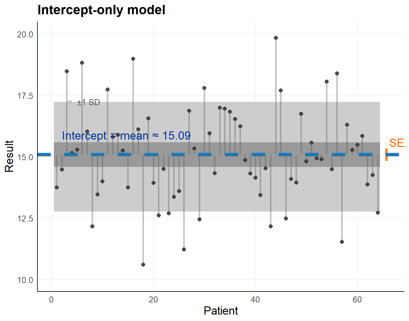
1.2 Regression Model: Mean and Variance

Regression as swiss knife.

A regression model with only an intercept extracts

mean (conditional on nothing else)
variance (of the residuals around the mean)
standard error (uncertainty around the estimated mean)

\[ y_i = \beta_0 + \varepsilon_i \qquad with \qquad \varepsilon_i \overset{\text{i.i.d.}}{\sim} \mathcal{N}(0, \sigma^2). \]

Patients on x-axis, observations on y-axis

line represents average
greyed band +/- 1 standard deviation

Fitted intercept is the mean,
or average SQUARE test result

\[ \hat{\beta}_0 = \bar{y} \]

Residuals are difference data - model based expectation.

\[ e_i = y_i - \bar{y} \]

No variance explained, with total variance \(\sigma^2\).

\[ \sigma^2 = \frac{1}{N} \sum_{i=1}^{N} (y_i - \mu)^2 \]

Predicts the same value for every case.

\[ SE(\hat{\beta}_0) = \frac{\sigma}{\sqrt{n}} \]

The standard error (SE; estimation) is a function of the standard deviation (sd; data).

lm_b0 <- lm(scores ~ 1, data = dta_base)

Term	Estimate	Std. Error	t value	p value
(Intercept)	15.086	0.251	60.221	2.11 × 10⁻⁵⁷

R²	adj. R²	σ	statistic	p.value	df	logLik	AIC	BIC	deviance	df.residual	nobs
0.000	0.000	2.004	NA	NA	NA	−134.801	273.601	277.919	253.034	63.000	64.000

1.3 Two Groups; t-test look-alike

A regression model with an intercept and a treatment effect (slope, dichotomous variable Treatment vs. Control)

treatment and control specific means
difference between treatment and control
standard error of difference

The regression model is:

\[ y_i = \beta_0 + \underline{\beta_1 x_i} + \varepsilon_i, \qquad \text{for } i = 1,\dots,n, \]

With

\[ x_i = \begin{cases} 0 & \text{for control}, \\ 1 & \text{for treatment}. \end{cases} \]

And the usual distributional assumptions.

\[ \varepsilon_i \overset{\text{i.i.d.}}{\sim} \mathcal{N}(0, \sigma^2). \]

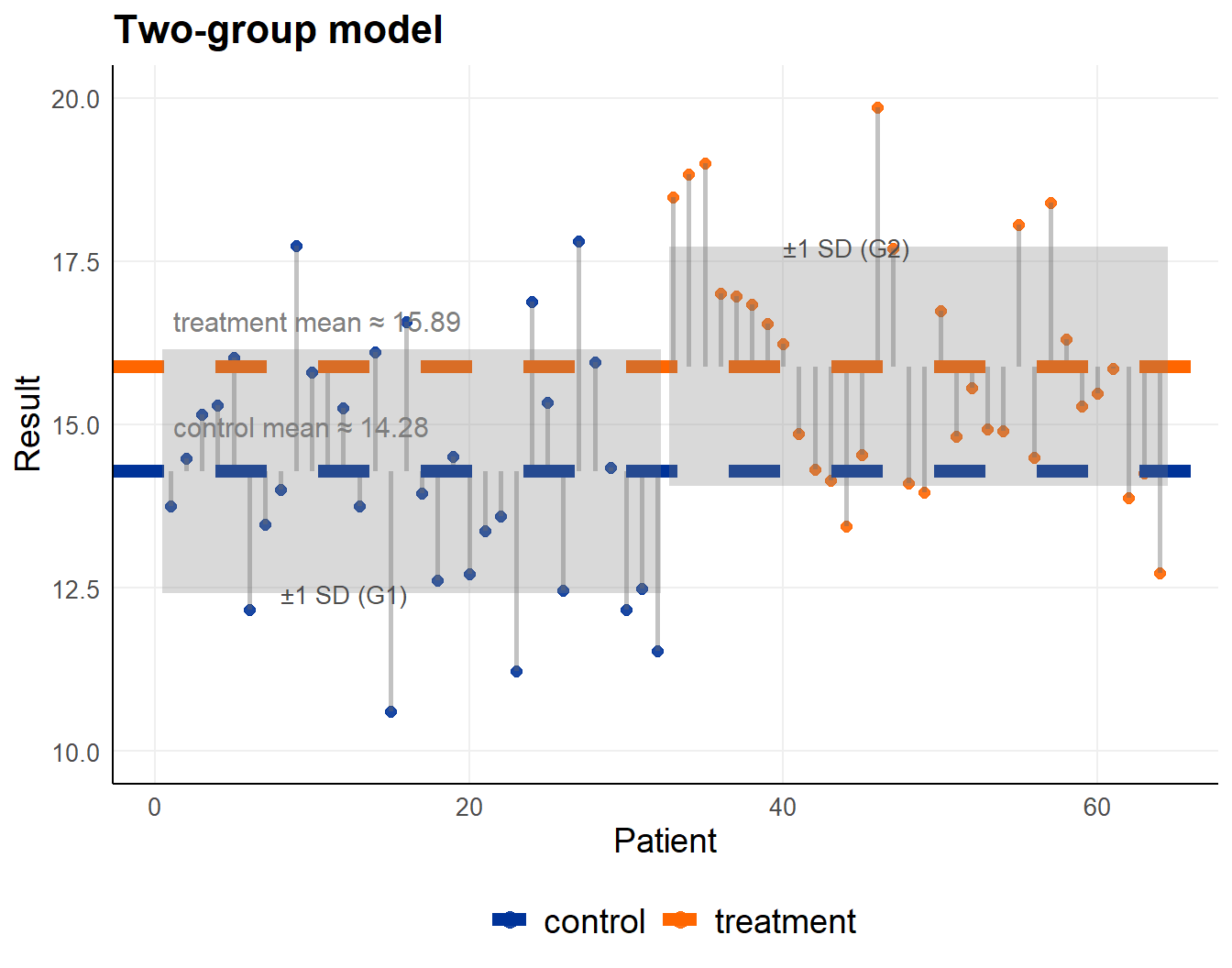
Patients on x-axis, observations on y-axis

line represents group specific means
greyed band +/- 1 group specific standard deviation

Fitted intercept is the mean for group coded as 0,
fitted slope is the difference between the two groups offer estimated group means (conditional means)

\[ \hat{\beta}_0 = \bar{y}_{x=0} \] \[ \hat{\beta}_1 = \bar{y}_{x=1} - \bar{y}_{x=0} \]

Residuals are still difference data - model based expectation.

\[ e_i = y_i - \hat{y}_i \]

Notice: residuals are defined over all observations, not per condition.

The standard error (SE; estimation) is a function of the group specific standard deviations (sd; data) and sample sizes.

About 16.36 % of the variance is now explained.

Predicts the same value for every case within a group.

lm_groups <- lm(score ~ group, data = dta_groups)

Term	Estimate	Std. Error	t value	p value
(Intercept)	14.282	0.327	43.728	2.62 × 10⁻⁴⁸
grouptreatment	1.609	0.462	3.483	9.15 × 10⁻⁴

R²	adj. R²	σ	statistic	p.value	df	logLik	AIC	BIC	deviance	df.residual	nobs
0.164	0.150	1.848	12.131	0.001	1.000	−129.082	264.165	270.641	211.627	62.000	64.000

1.4 Continuous Variable

A regression model with an intercept and a continuous predictor (slope)

predictor specific means
difference for 1 unit extra on the predictor
standard error of the slope

The regression model is exactly the same as before:

\[ y_i = \beta_0 + \underline{\beta_1 x_i} + \varepsilon_i, \qquad \text{for } i = 1,\dots,n, \]

with the usual distributional assumption:

\[ \varepsilon_i \overset{\text{i.i.d.}}{\sim} \mathcal{N}(0, \sigma^2). \]

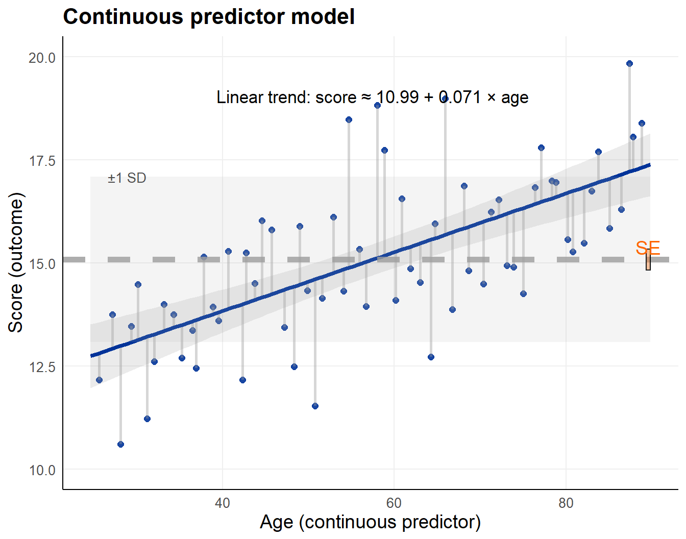
Figure 3: Predictor value specific means

Note, the same 64 scores are used, but treated as continuous predictor \(x_i\).

Predictor \(x_i\) on x-axis (age), observations on y-axis

line represents linear trend
greyed band +/- 1 overall standard deviation

Fitted intercept is the mean at \(x_i\) = 0
Fitted slope is increase per unit \(x_i\),

Note: center your \(x_i\) around another value,
change the intercept.

\[ \hat{\beta}_0 = \mathbb{E}[Y \mid X=0] \]

\[ \hat{\beta}_1 = \frac{\Delta \mathbb{E}[Y]}{\Delta X} \]

Residuals are difference
data - model based expectation.

\[ e_i = y_i - \hat{y}_i \]

\[ SE(\hat{\beta}_1) = \sqrt{\frac{sd^2}{n \cdot \text{Var}(X)}} \]

The standard error (SE; estimation) is a function of the residual variance relative to predictor spread.

lm_cont <- lm(score ~ age, data = dta_cont)

Term	Estimate	Std. Error	t value	p value
(Intercept)	10.987	0.618	17.770	5.15 × 10⁻²⁶
age	0.071	0.010	6.963	2.49 × 10⁻⁹

R²	adj. R²	σ	statistic	p.value	df	logLik	AIC	BIC	deviance	df.residual	nobs
0.439	0.430	1.513	48.484	0.000	1.000	−116.313	238.626	245.103	141.995	62.000	64.000

1.5 Dichotomized continuous predictor

Same model !

A regression model with an intercept and a continuous predictor that is dichotomized into two groups.

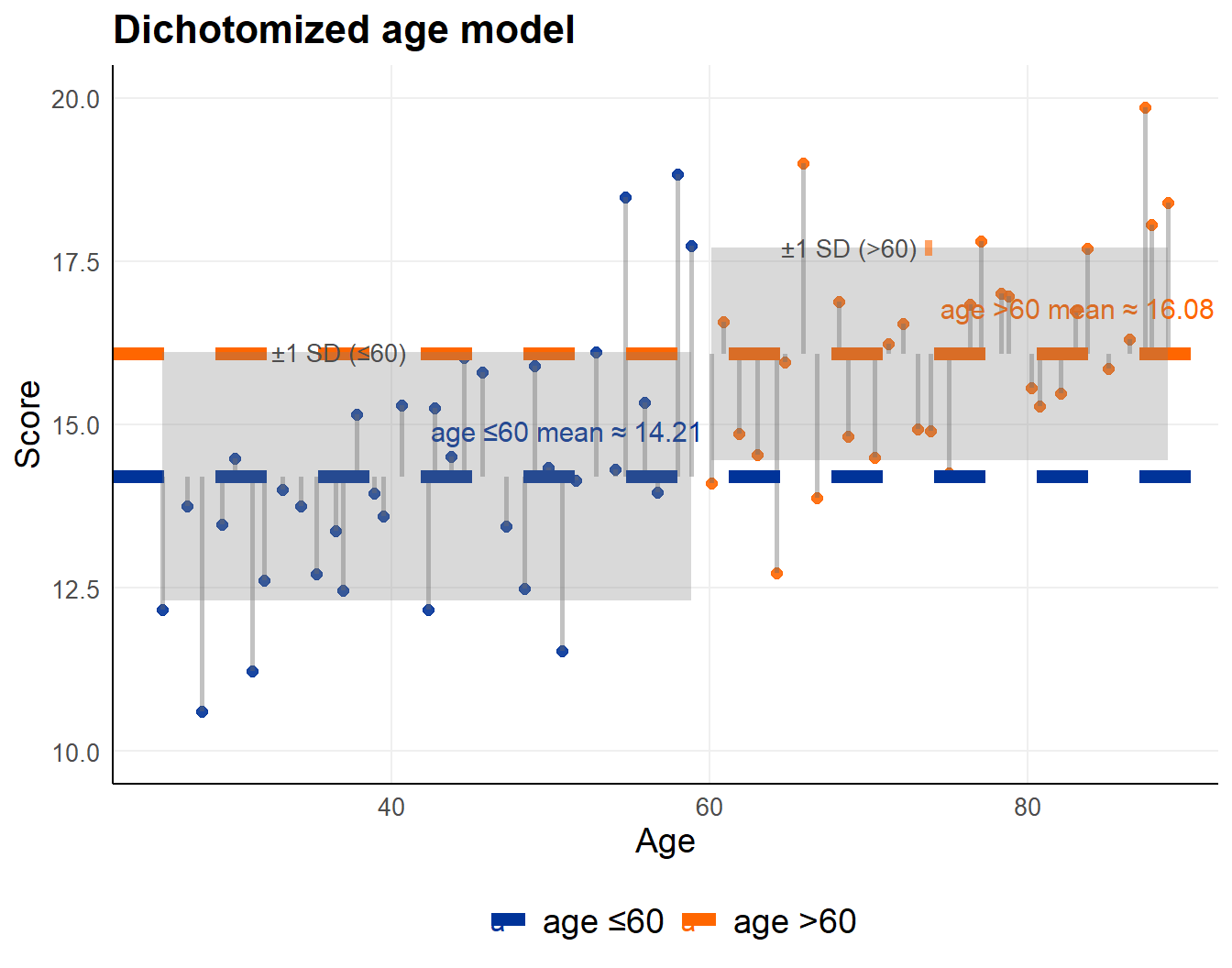
Predictor \(X_i\) on x-axis (age), observations on y-axis

line represents group specific average
greyed band +/- 1 group specific standard deviation

Same model, but

residual variance increases
explained variance decreases
residuals are clustered, not independent

violation of the distributional assumption:

\[ \varepsilon_i \overset{\text{i.i.d.}}{\sim} \mathcal{N}(0, \sigma^2). \]

lm_dich <- lm(score ~ age_d, data = dta_dich)

Term	Estimate	Std. Error	t value	p value
(Intercept)	14.206	0.306	46.487	6.59 × 10⁻⁵⁰
age_dage >60	1.877	0.446	4.206	8.51 × 10⁻⁵

R²	adj. R²	σ	statistic	p.value	df	logLik	AIC	BIC	deviance	df.residual	nobs
0.222	0.209	1.782	17.692	0.000	1.000	−126.767	259.535	266.011	196.858	62.000	64.000

1.6 Multiple Regression; combining information

A regression model with an intercept, a group difference, and a continuous predictor

predictor specific means
that can differ depending on other predictors
with standard errors for each slope

The regression model starts being interesting:

\[ y_i = \beta_0 + \beta_1 x_{1i} + \beta_2 x_{2i} + \beta_3 x_{1i} x_{2i} + \varepsilon_i, \qquad \text{for } i = 1,\dots,n, \]

with the usual distributional assumption:

\[ \varepsilon_i \overset{\text{i.i.d.}}{\sim} \mathcal{N}(0, \sigma^2). \]

1.6.1 Interaction

Interactions would allow effects to be condition dependent.

Age effect differs per group.
Group difference are age dependent.

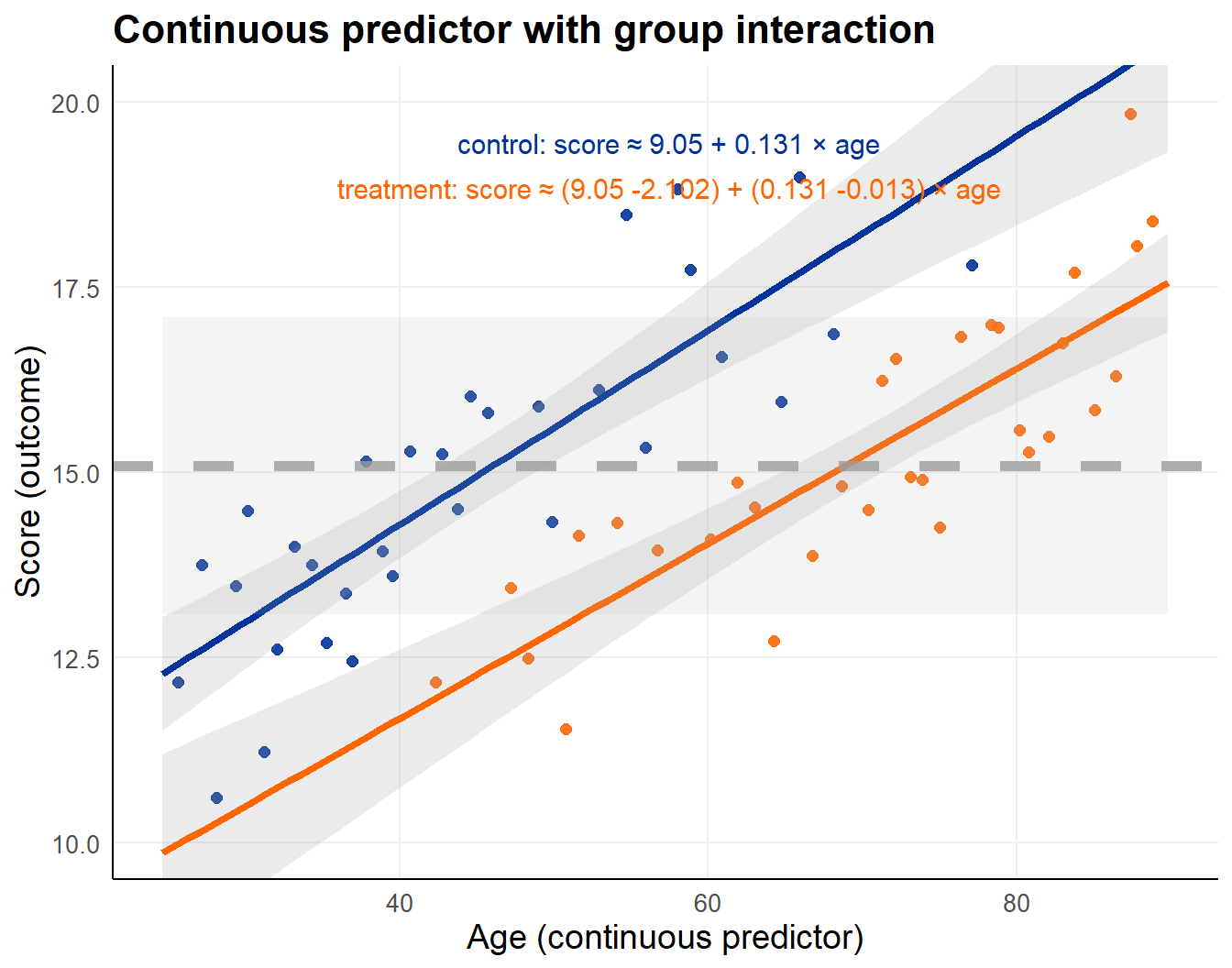
Predictor \(x_{2i}\) on x-axis (age), observations on y-axis

line represents group specific linear trend
greyed band +/- 1 group specific standard deviation

lm_int <- lm(score ~ age * group, data = dta_int)

Term	Estimate	Std. Error	t value	p value
(Intercept)	9.050	0.684	13.227	1.94 × 10⁻¹⁹
age	0.131	0.015	8.942	1.24 × 10⁻¹²
grouptreatment	−2.102	1.266	−1.660	1.02 × 10⁻¹
age:grouptreatment	−0.013	0.021	−0.620	5.38 × 10⁻¹

In this case, no evidence for an interaction.

R²	adj. R²	σ	statistic	p.value	df	logLik	AIC	BIC	deviance	df.residual	nobs
0.707	0.692	1.112	48.215	0.000	3.000	−95.539	201.077	211.872	74.187	60.000	64.000

1.6.2 Main effects

Simplifying the model and its interpretation, the interaction is removed.

When age is considered jointly with group.

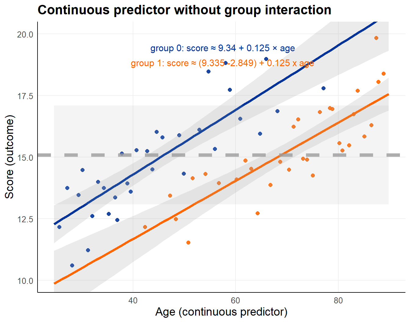
Predictor \(x_{2i}\) on x-axis (age), observations on y-axis

line represents group specific linear trend
greyed band +/- 1 group specific standard deviation

lm_int_main <- lm(score ~ age + group, data = dta_int)

Term	Estimate	Std. Error	t value	p value
(Intercept)	9.335	0.504	18.527	9.82 × 10⁻²⁷
age	0.125	0.010	12.005	1.04 × 10⁻¹⁷
grouptreatment	−2.849	0.384	−7.417	4.44 × 10⁻¹⁰

There is a very clear group effect. In this case, no evidence for an interaction.

R²	adj. R²	σ	statistic	p.value	df	logLik	AIC	BIC	deviance	df.residual	nobs
0.705	0.695	1.106	72.866	0.000	2.000	−95.743	199.486	208.122	74.662	61.000	64.000

1.6.3 Ignoring a relevant predictor

With only group in the model, ignoring age.

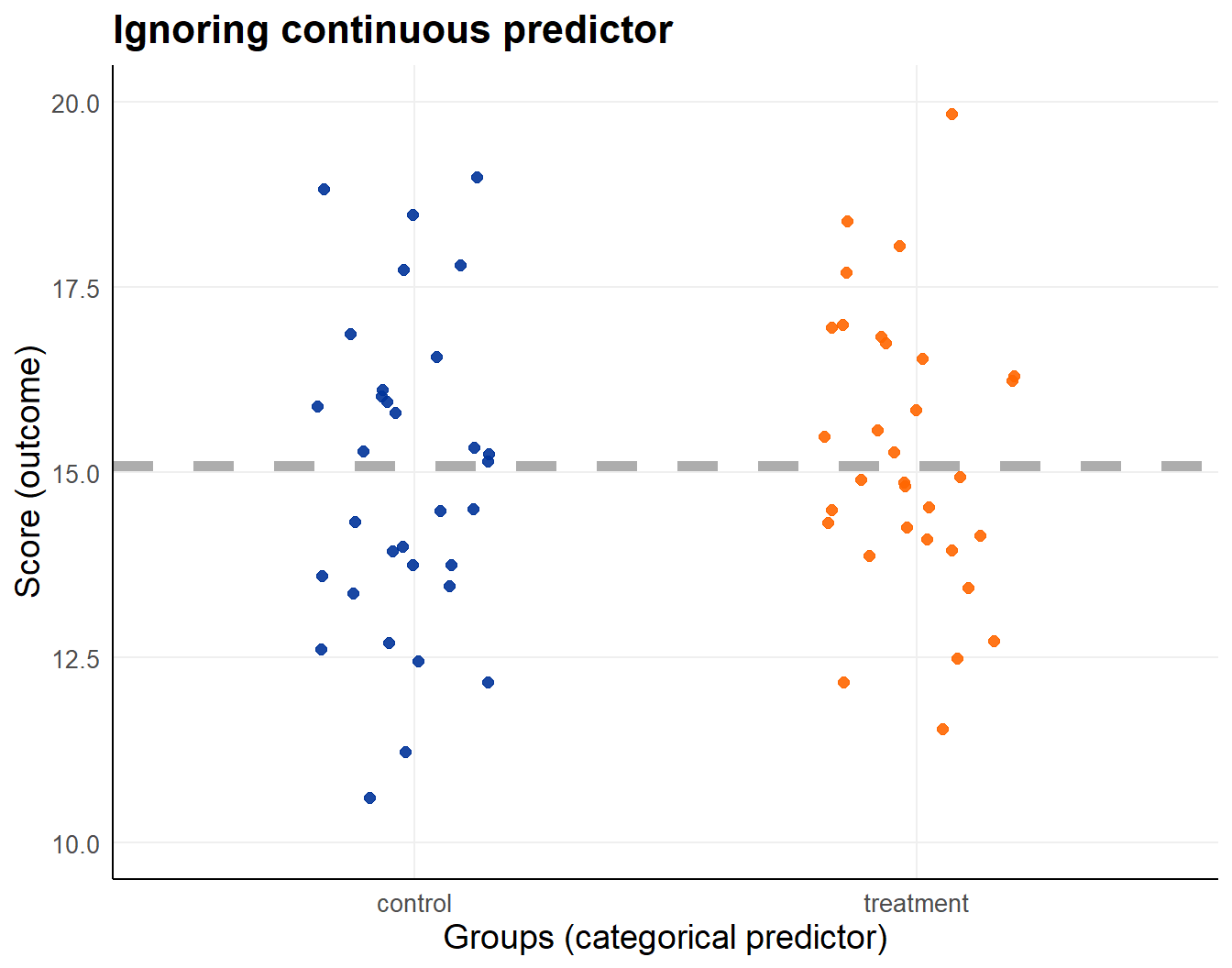
Predictor \(x_{1i}\) on x-axis (age), observations on y-axis

lm_int_ign <- lm(score ~ group, data = dta_int)

Term	Estimate	Std. Error	t value	p value
(Intercept)	14.910	0.356	41.915	3.32 × 10⁻⁴⁷
grouptreatment	0.351	0.503	0.698	4.88 × 10⁻¹

There is no group effect !
Remember: conditional on age there is one.

Do not make decisions based on univariable analysis unless you have to.

R²	adj. R²	σ	statistic	p.value	df	logLik	AIC	BIC	deviance	df.residual	nobs
0.008	−0.008	2.012	0.487	0.488	1.000	−134.550	275.100	281.577	251.061	62.000	64.000

1.7 Assumptions

Models are based on assumptions,
violations can compromise inference.

For linear regression the assumptions are:

Linearity: Predictor-outcome relationship is linear
Independence: Residuals are i.i.d. (no clustering/autocorrelation)
Homoscedasticity: Constant residual variance
Normality: Residuals normally distributed (for inference)

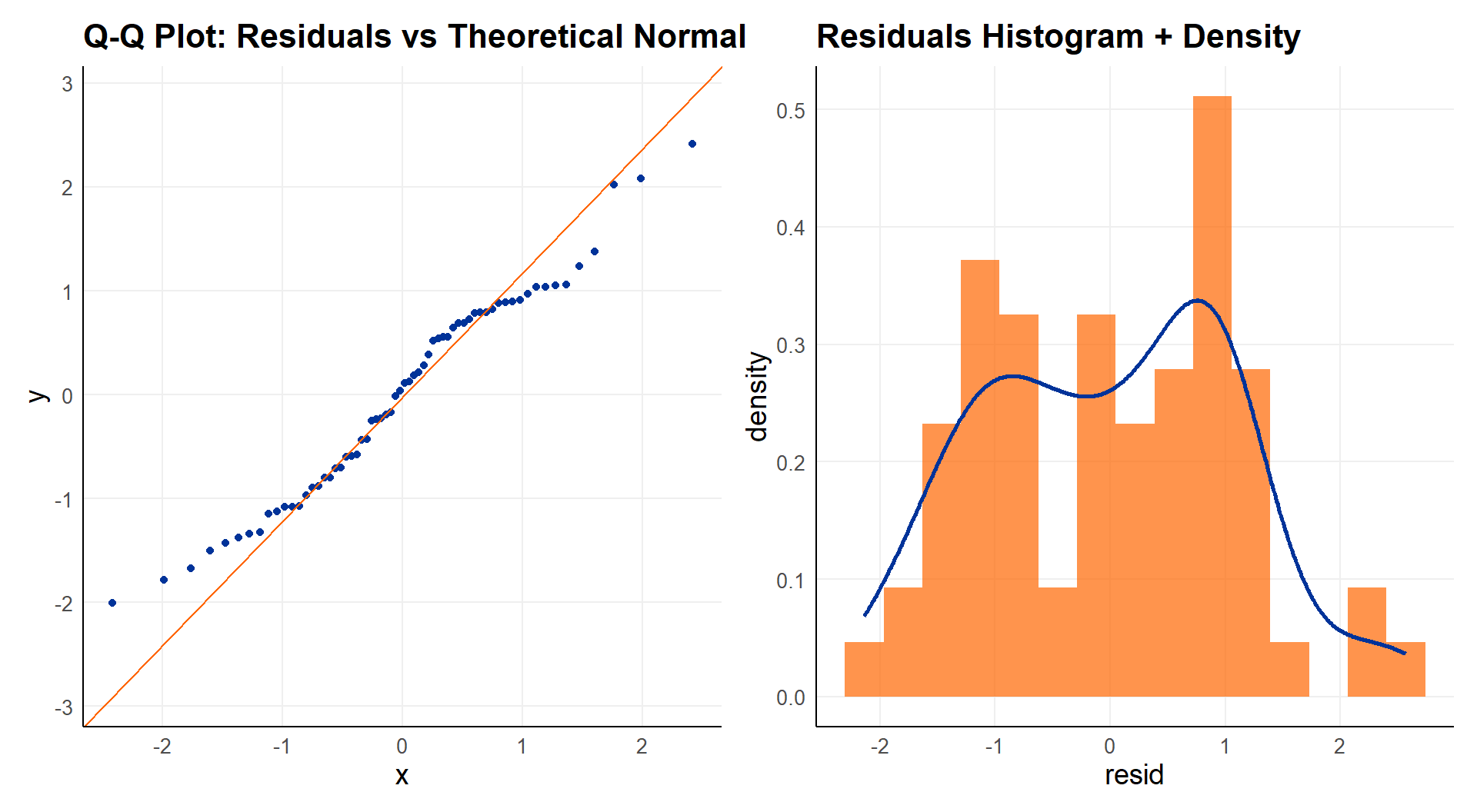
Evaluation of model assumption is based on (standardized) residuals.

To evaluate linearity, plot the outcome in relation to

the fitted value for the whole model
individual predictors for parts of the model

To evaluate independence, plot the residuals in relation to

the fitted value for the whole model
individual predictors for parts of the model

and watch out for patterns

To evaluate homoscedasticity, plot the standardized residuals in relation to

individual predictors for parts of the model

and watch out for predictor specific spread

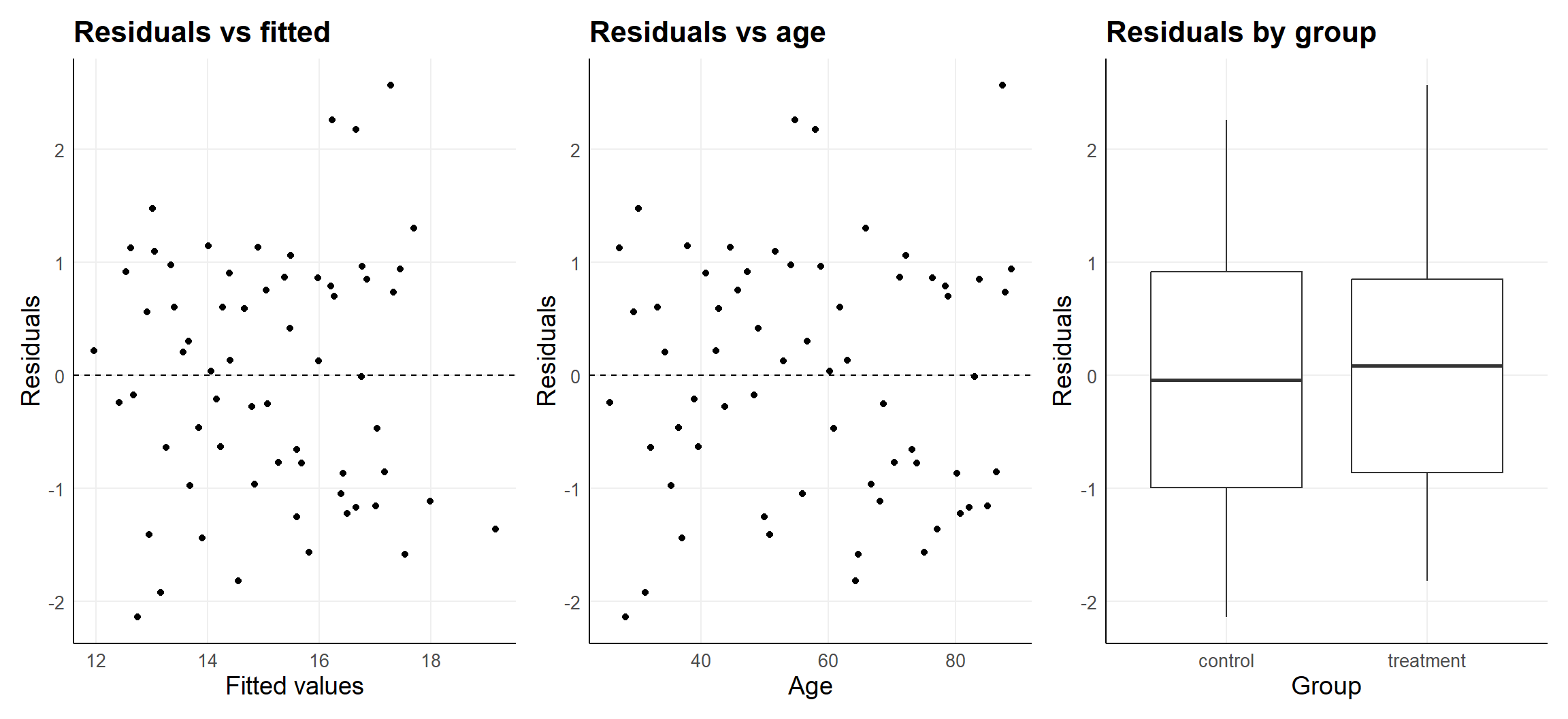
To evaluate normality of the residuals, use a qqplot.
Note, normality of (standardized) residuals follows from the assumption that disturbances are random and additive.

For the identically and individually distributed assumption:

\[\varepsilon_i \overset{\text{i.i.d.}}{\sim} \mathcal{N}(0, \sigma^2). \]

The lack of any patterns supports the i.i.d. assumption (does not prove it) Remaining patterns in the residuals can possibly be addressed

using additional variables
using transformations

Build models to capture the systematicity in the data,
so the remaining part is random, and ideally relatively small.

For completeness,
while tests are just tests:

Diagnostics Tests
Test	Result	Interpretation
Durbin-Watson (Independence)	2.030	≈2 = no autocorrelation ✓
Breusch-Pagan (Homoscedasticity)	0.257	p > 0.05 = constant variance ✓
Shapiro-Wilk (Normality)	0.162	p > 0.05 = normality ✓

2 Dependent data

Data is often internally dependent:

cross-sectional clustering: groups of observations (classes, litters, clinics, …)
within-unit clustering: repeated measures (trajectories, pre-post, …)
distances (less relation when further)
study effects measuring the same (meta-analysis)
spatial random effects
item response models, with respondent clustering
…

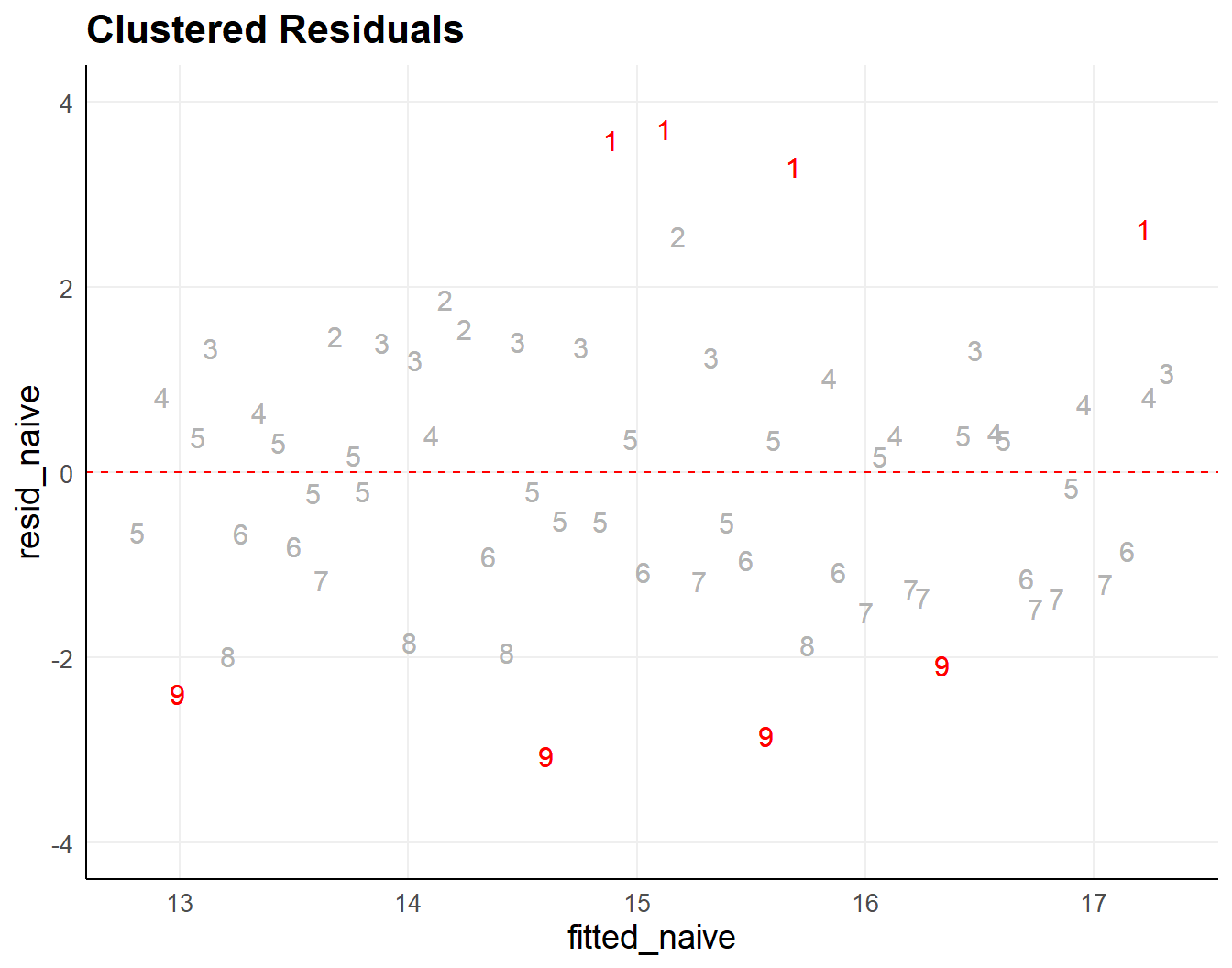
What dependency looks like:

Note the assumption

\[ \varepsilon_i \overset{\text{i.i.d.}}{\sim} \mathcal{N}(0, \sigma^2). \]

All residuals (variance unaccounted for by the model) assumed distributed individually and identically,
all part of the same underlying distribution !

Any residual is fully uninformative about any other residual. All residuals combined reflect one single distribution.

The clustering shows that grouping should be included in the model.

2.1 Working Example

Let’s assume a SQUARE test exists

with test results between 0 and 20
performed on patients
part of one of 9 groups of patients
who have particular characteristics (e.g., age, …)
under particular conditions (e.g., treated or not)

We want to understand the conditions (e.g., treatment) under which test results are higher/lower

acknowledging group-members to be more similar to each-other, in average
by relating
- the data (test results ~ outcome) to
- the conditions (patient properties ~ predictors)
- → columns
using information offered by each of the patients (replications ~ sample size)
- → rows

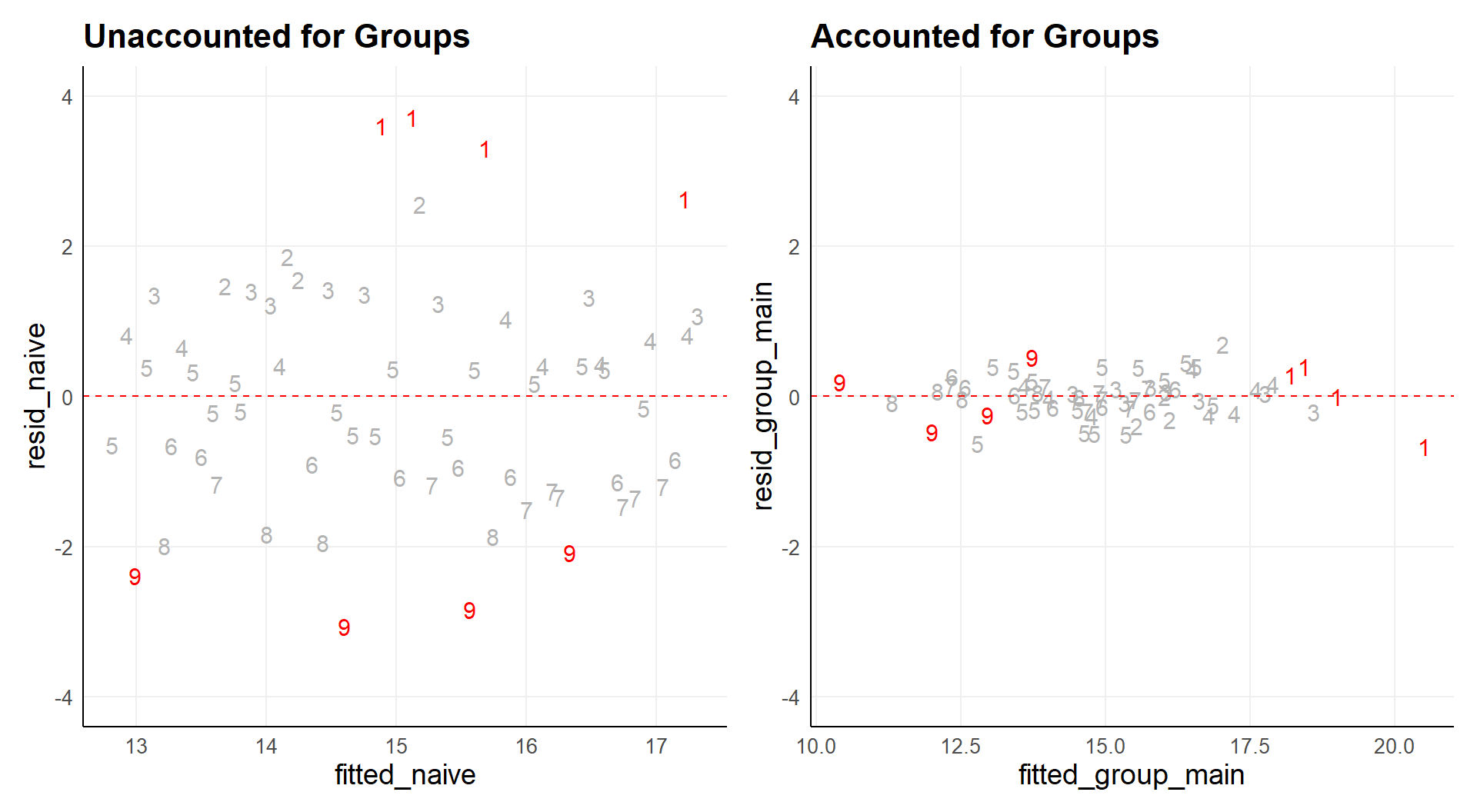
2.2 Regression Model: grouping as Fixed variable

Bringing in groups

reduces residuals
results in residuals around 0 for each group
removed dependence: knowledge of an instance of a group is not informative about the other instances

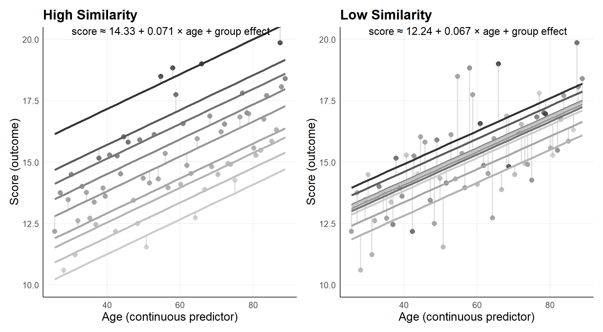
2.2.1 Independent groups, common age effect

Using a group identification variable to account for groups.

The regression model is the same as before, 9 groups instead of 2:

\[ y_i = \beta_0 + \beta_1 x_i + \underline{\beta_2 g_i} + \varepsilon_i, \qquad \text{for } i = 1,\dots,n, \]

with the usual distributional assumption:

\[ \varepsilon_i \overset{\text{i.i.d.}}{\sim} \mathcal{N}(0, \sigma^2). \]

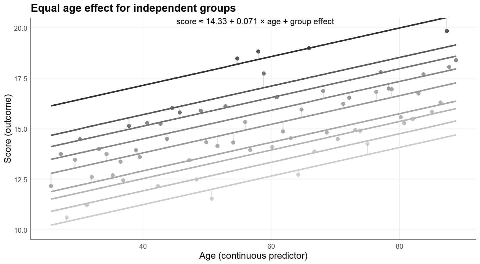
Figure 11: Grouping as Fixed Variable; Age effect considered equal over groups, high within group similarity

Age effect, assumed equal for each of 9 groups.

Age on x-axis, observations on y-axis

lines represent group specific conditional averages
- in this case, conditional on age
- age effect, independent of group

With nine groups in the model.

lm_group_main_9 <- lm(score ~ age + group, data = dta_grouped)

Term	Estimate	Std. Error	t value	p value
(Intercept)	14.327	0.213	67.238	9.56 × 10⁻⁵⁴
age	0.071	0.002	31.777	1.24 × 10⁻³⁶
group2	−1.458	0.221	−6.606	1.80 × 10⁻⁸
group3	−2.021	0.189	−10.696	5.99 × 10⁻¹⁵
group4	−2.652	0.188	−14.133	8.70 × 10⁻²⁰
group5	−3.347	0.174	−19.287	6.97 × 10⁻²⁶
group6	−4.245	0.188	−22.564	3.66 × 10⁻²⁹
group7	−4.623	0.188	−24.652	4.66 × 10⁻³¹
group8	−5.230	0.221	−23.711	3.20 × 10⁻³⁰
group9	−5.914	0.218	−27.133	3.84 × 10⁻³³

R²	adj. R²	σ	statistic	p.value	df	logLik	AIC	BIC	deviance	df.residual	nobs
0.980	0.977	0.306	294.448	0.000	9.000	−9.568	41.136	64.884	5.053	54.000	64.000

There is a clear age and group effect, each of the groups differs from the reference group conditional on age.
The Mean Squared Error is huge compared to the Residual Variance.

Term	df	Sum Sq	Mean Sq	F value	p value
age	1.000	111.039	111.039	1,186.612	1.95 × 10⁻³⁸
group	8.000	136.942	17.118	182.928	2.80 × 10⁻³⁶
Residuals	54.000	5.053	0.094	NA	NA

2.2.2 Group specific age effect

What if we would allow group specific age effects.

The regression model is:

\[ y_i = \beta_0 + \beta_1 \cdot x1_i + \beta_2 \cdot g2_i + \beta_3 \cdot x1_i \cdot g2_i + \varepsilon_i, \qquad \text{for } i = 1,\dots,n, \]

with the usual distributional assumption:

\[ \varepsilon_i \overset{\text{i.i.d.}}{\sim} \mathcal{N}(0, \sigma^2). \]

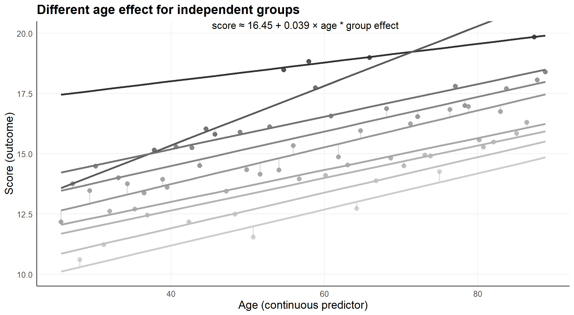
Figure 12: Grouping as Fixed Variable; Age effect allowed to be different over groups, high within group similarity

The age effect is allowed to differ for each of 9 groups.

Age on x-axis, observations on y-axis

lines represent group specific conditional averages

With nine group in the model.

lm_group_int_9 <- lm(score ~ age * group, data = dta_grouped)

Term	Estimate	Std. Error	t value	p value
(Intercept)	16.453	0.730	22.541	1.69 × 10⁻²⁶
age	0.039	0.011	3.611	7.51 × 10⁻⁴
group2	−6.047	1.123	−5.386	2.38 × 10⁻⁶
group3	−3.964	0.793	−5.001	8.75 × 10⁻⁶
group4	−4.818	0.785	−6.141	1.78 × 10⁻⁷
group5	−5.759	0.762	−7.560	1.33 × 10⁻⁹
group6	−6.099	0.798	−7.643	9.98 × 10⁻¹⁰
group7	−6.496	0.872	−7.447	1.95 × 10⁻⁹
group8	−7.488	0.897	−8.347	9.14 × 10⁻¹¹
group9	−8.260	0.857	−9.640	1.29 × 10⁻¹²
age:group2	0.085	0.021	4.033	2.06 × 10⁻⁴
age:group3	0.029	0.012	2.384	2.13 × 10⁻²
age:group4	0.033	0.012	2.803	7.39 × 10⁻³
age:group5	0.037	0.011	3.259	2.11 × 10⁻³
age:group6	0.027	0.012	2.281	2.73 × 10⁻²
age:group7	0.028	0.013	2.240	3.00 × 10⁻²
age:group8	0.035	0.015	2.293	2.65 × 10⁻²
age:group9	0.036	0.013	2.702	9.61 × 10⁻³

R²	adj. R²	σ	statistic	p.value	df	logLik	AIC	BIC	deviance	df.residual	nobs
0.986	0.981	0.274	194.902	0.000	17.000	2.507	32.986	74.005	3.465	46.000	64.000

There is a clear age and group effect, each of the groups differs from the reference group conditional on age.
The Mean Squared Error is huge compared to the Residual Variance.

Term	df	Sum Sq	Mean Sq	F value	p value
age	1.000	111.039	111.039	1,474.179	1.36 × 10⁻³⁶
group	8.000	136.942	17.118	227.259	2.55 × 10⁻³⁴
age:group	8.000	1.588	0.199	2.636	1.82 × 10⁻²
Residuals	46.000	3.465	0.075	NA	NA

2.3 Regression Model: Why this sometimes is not enough

Grouping as fixed variable can be a problem,
especially with many small clusters (groups):

many parameters have to be estimated because many clusters
for each cluster, parameters poorly estimated when small clusters (overfitting)
no generalization to clusters not part of the data

Ignoring grouping is a problem when within group similarities exist (dependencies):

violation of i.i.d. assumption
Standard errors are too small → p-values too small → false positives inflate.
group specific effects ignored too

Solution: model the within group similarities,
once estimated the rest of the model is conditional upon it.

2.4 Note: within cluster similarity ~ between cluster difference

Capture dependence through estimating variance.

Figure 14: Variance and Correlation, two sides of a coin

3 Mixed Model

Mixed models (a.k.a Multilevel Model)

extend regression models,
is modeling variance
turning it into a conditional mean
by estimating relations
by minimizing squared error.
while accomodating dependencies
through estimating variances (heterogeneity)

3.1 Random Intercept Model

Let \(y_{ij}\) denote the outcome for individual \(i\) in cluster \(j\).

Level 1 (case within cluster): \[ y_{ij} = \underline{\beta_{0j}} + \beta_1 x_{ij} + \varepsilon_{ij}, \qquad \varepsilon_{ij} \sim \mathcal{N}(0,\ \sigma^2) \]

Level 2 (cluster-level model for the intercept): \[ \underline{\beta_{0j}} = \gamma_{00} + u_{0j}, \qquad u_{0j} \sim \mathcal{N}(0,\ \tau_{00}) \]

Combined (reduced form): \[ y_{ij} = \underbrace{\gamma_{00} + \beta_1 x_{ij}}_{\text{fixed part}} + \underbrace{u_{0j} + \varepsilon_{ij}}_{\text{random part}} \]

The random part implies a variance decomposed into random intercept variance and residual variance:

\[ \text{Var}(y_{ij}) = \tau_{00} + \sigma^2, \qquad \text{Cov}(y_{ij},\ y_{i'j}) = \tau_{00} \quad (i \neq i', \text{ same group } j) \]

The relative proportion of heterogeity for this simple model is the intra class correlation (ICC):

\(\text{ICC} = \tau_{00} / (\tau_{00} + \sigma^2)\).

3.2 Why a Random Intercept Model

Mixed models treat cluster effects as random draws from a distribution.

Instead of estimating J-1 fixed effects + intercept

\[ \beta_{0}, \beta_{1}, ..., \beta_{J-1} \]

random effects are estimated as

\[ \gamma_{00} + u_{0j} \qquad with \qquad u_{0j} \sim \mathcal{N}(0,\ \tau_{00}) \]

resulting in only 2 parameters to estimate: grand mean \(\gamma_{00}\) and variance \(\tau_{00}\)

Notice the similarity with the residuals:

\[ \varepsilon_i \overset{\text{i.i.d.}}{\sim} \mathcal{N}(0, \sigma^2). \]

A single variance parameter captures cluster heterogeneity

With a growing number of clusters

no increase in number of parameters to estimate
a better estimate of the variance parameter

In this particular case:

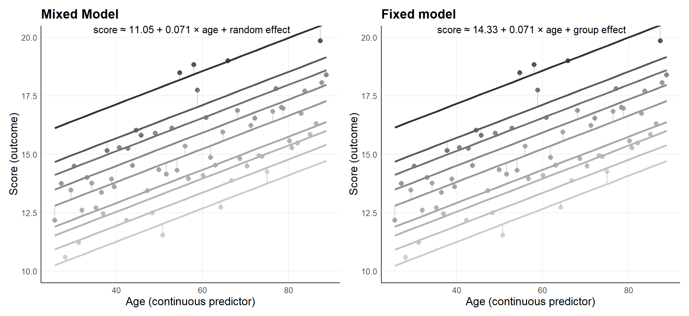
Mixed
in R:
lmer(score ~ age + (1 | group),
data = ..)

term	estimate	std.error	df	statistic
(Intercept)	11.049	0.652	8.621	16.943
age	0.071	0.002	54.054	31.797
sd__(Intercept)	1.914	NA	NA	NA
sd__Observation	0.306	NA	NA	NA

Cluster specific estimates extracted:

(Intercept)
3.25578815
1.80731994
1.25143614
0.62302063
-0.07019019
-0.96517266
-1.34190800
-1.94038853
-2.61990547

metric	icc_vals
tau_00	3.6648637
sigma2	0.0935955
ICC	0.9750974

Fixed
in R
lm(score ~ age + group,
data = ..)

term	estimate	std.error	statistic
(Intercept)	14.327	0.213	67.238
age	0.071	0.002	31.777
group2	-1.458	0.221	-6.606
group3	-2.021	0.189	-10.696
group4	-2.652	0.188	-14.133
group5	-3.347	0.174	-19.287
group6	-4.245	0.188	-22.564
group7	-4.623	0.188	-24.652
group8	-5.230	0.221	-23.711
group9	-5.914	0.218	-27.133

Fixed, residuals

sigma
0.306

3.3 Level specific slopes

Different levels can have different predictors of the observations (at level 1).

example: test results explained by patient (level 1) hospital (level 2) variables
- e.g., older patients (age) result in higher scores
- e.g., university hospitals (type) result in higher scores

Note: Variables can only explain variability at the lower or equal level.

Let \(y_{ij}\) denote the outcome for individual \(i\) in cluster \(j\).

Level 1 (case within cluster): \[ y_{ij} = \beta_{0j} + \beta_{1} x_{ij} + \varepsilon_{ij}, \qquad \varepsilon_{ij} \sim \mathcal{N}(0,\ \sigma^2) \]

Level 2 (cluster-level model for the intercept, with a Level‑2 predictor \(z_{j}\)): \[ \beta_{0j} = \gamma_{00} + \underline{\gamma_{01} z_{j}} + u_{0j}, \qquad u_{0j} \sim \mathcal{N}(0,\ \tau_{00}) \]

Combined (reduced form): \[ y_{ij} = \underbrace{\gamma_{00} + \beta_{1} x_{ij} + \gamma_{01} z_{j}}_{\text{fixed part}} + \underbrace{u_{0j} + \varepsilon_{ij}}_{\text{random part}} \]

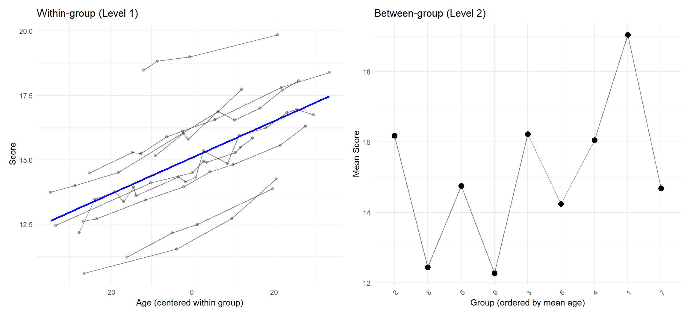
The same variable can sometimes be split up and defined at different levels. Let \(y_{ij}\) denote the outcome for individual \(i\) in cluster \(j\).

Level 1 (case within cluster): \[ y_{ij} = \beta_{0j} + \underline{\beta_{1W} x_{ijW}} + \varepsilon_{ij}, \qquad \varepsilon_{ij} \sim \mathcal{N}(0,\ \sigma^2) \]

where
\(x_{ijW} = x_{ij} - \bar{x}_{j}\) (within-cluster centered \(x\))
\(\bar{x}_{j} = \frac{1}{n_j}\sum_{i=1}^{n_j} x_{ij}\) (cluster mean of \(x\))

Level 2 (cluster-level model for the intercept, now including the cluster mean): \[ \beta_{0j} = \gamma_{00} + \underline{\gamma_{01}\bar{x}_{j}} + u_{0j}, \qquad u_{0j} \sim \mathcal{N}(0,\ \tau_{00}) \]

Combined (reduced form): \[ y_{ij} = \underbrace{\gamma_{00} + \beta_{1W} x_{ijW} + \gamma_{01}\bar{x}_{j}}_{\text{fixed part}} + \underbrace{u_{0j} + \varepsilon_{ij}}_{\text{random part}} \]

A fixed slope, maybe age, or weight, … split in

within cluster centered slope
cluster specific average

One part focusses on within cluster relative position, other on cluster properties.

Example: blood pressure explained by body weight

patients with relatively higher weights in a hospital may have higher blood pressure
hospitals may differ in average weight because of …

Without this split, it could be a blend.

Note: ecological fallacy.

Figure 16: Within and Between Group Differences

Repeating just fitting a slope.

effect	group	term	estimate	std.error	statistic	df	p.value
fixed	NA	(Intercept)	11.0488	0.6521	16.9431	8.6207	0
fixed	NA	age	0.0709	0.0022	31.7967	54.0537	0
ran_pars	group	sd__(Intercept)	1.9144	NA	NA	NA	NA
ran_pars	Residual	sd__Observation	0.3059	NA	NA	NA	NA

nobs	sigma	logLik	AIC	BIC	REMLcrit	df.residual
64	0.306	-43.568	95.136	103.771	87.136	60

Splitting up over levels.

effect	group	term	estimate	std.error	statistic	df	p.value
fixed	NA	(Intercept)	8.8772	5.1324	1.7296	6.9933	0.1274
fixed	NA	agem	0.1089	0.0890	1.2233	6.9917	0.2609
fixed	NA	agec	0.0709	0.0022	31.7744	53.9835	0.0000
ran_pars	group	sd__(Intercept)	2.0212	NA	NA	NA	NA
ran_pars	Residual	sd__Observation	0.3059	NA	NA	NA	NA

nobs	sigma	logLik	AIC	BIC	REMLcrit	df.residual
64	0.306	-44.999	99.997	110.792	89.997	59

For the data, a general slope can be fitted, and alternatively, a within and a between slope.

Relative age matters within clusters,
Cluster average ages does not matter.

3.4 Borrowing Strength: Partial Pooling

Strategies for estimating each clusters’ intercept:

No pooling: independent clusters, ignores information from other clusters
Complete pooling: grand mean, ignores group membership
Partial pooling: reconciles both, compromise

Partial pooling, the key mixed model characteristic

cluster specific estimates
more global estimates

Possible becasue clusters sampled from an underlying population

other clusters are informative
use dependency through common population of clusters

Partial pooling implies shrinkage:
shrink each group estimate toward the grand mean
results in random effects \(\hat{u}_{0j}\) or Best Linear Unbiased Predictor (BLUP):

\[ \hat{u}_{0j} = \underbrace{\frac{n_j/\sigma^2}{n_j/\sigma^2 + 1/\tau_{00}}}_{\text{reliability weight}\ \lambda_j} \cdot \left(\bar{y}_{\cdot j} - \hat{\gamma}_{00}\right) \]

The weight defines the percentage with which cluster specific deviation from the global average shrink

\(\lambda_j \to 1\) with increasing cluster sizes and stronger within cluster correlations (trust the raw data)
\(\lambda_j \to 0\) witch decreasing cluster sizes and weaker within cluster correlations (shrink toward the overall mean).

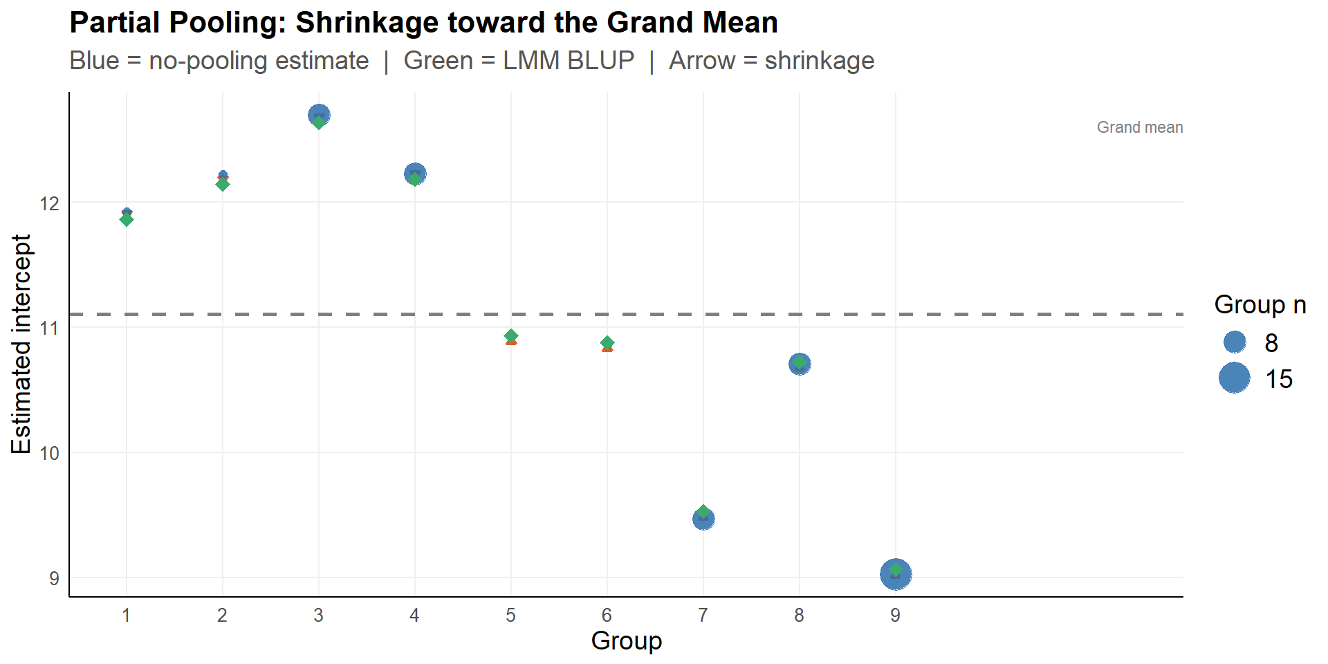
Figure 17: Partial pooling. blue = no-pooling, green = LMM BLUPs

Note: modeling the correlation to shrink estimates allows for cluster specific effects not explicitely represented

Example: matching is not a reason to turn to mixed models,
matching uses explicitly available information that should included in the model as such

3.5 Within-Cluster Correlation and Effective Sample Size

Consider two types of predictors:

Between-cluster predictor \(Z_j\) (e.g. hospital type)
- Only varies between clusters, constant within a cluster.
Within-cluster predictor \(x_{ij}\) (e.g. treatment dose)
- Varies within clusters.

For a balanced design with \(J\) clusters and \(m\) observations per cluster:

Variance of the estimator for the between-cluster effect is approximately proportional to

\[ \text{Var}(\hat{\gamma}_{01}) \propto \frac{\tau_{00} + \sigma^2/m}{J}. \]

Variance of the estimator for the within-cluster effect is approximately proportional to

\[ \text{Var}(\hat{\gamma}_{10}) \propto \frac{\sigma^2}{J \cdot m}. \]

As \(\rho\) increases (i.e. \(\tau_{00}\) grows relative to \(\sigma^2\)):

\(\tau_{00} + \sigma^2/m\) becomes larger \(\Rightarrow\) between-cluster effects become harder to detect.
\(\sigma^2\) becomes smaller relative to the total variance \(\Rightarrow\) within-cluster effects become easier to detect.

Stronger within-cluster correlation makes

between-cluster differences harder to detect.
within-cluster differences easier to detect.

Note: cluster randomization focuses on between cluster effects, dependent more on the number of clusters, less on the number of observations.

To compare treatments,
randomizing within each cluster is usually far more efficient

3.6 Adding a Random Slope

3.6.1 Heterogeneity of Effects

A cluster specific slope (effect) can be considered sampled from a common population, with a mean and variance. This is equivalent to cluster specific intercepts.

Level 1: \[ y_{ij} = \beta_{0j} + \underline{\beta_{1j} x_{ij}} + \varepsilon_{ij}, \qquad \varepsilon_{ij} \sim \mathcal{N}(0,\ \sigma^2) \]

Level 2: \[ \beta_{0j} = \gamma_{00} + u_{0j}, \qquad \underline{\beta_{1j}} = \gamma_{10} + u_{1j} \]

Distributional assumption for the random effects: \[ \begin{pmatrix} u_{0j} \\ u_{1j} \end{pmatrix} \sim \mathcal{N}\!\left(\begin{pmatrix}0\\0\end{pmatrix},\ \boldsymbol{\Psi}\right), \qquad \boldsymbol{\Psi} = \begin{pmatrix} \underline{\tau_{00}} & \underline{\tau_{01}} \\ \tau_{01} & \underline{\tau_{11}} \end{pmatrix} \]

Combined: \[ y_{ij} = \underbrace{\gamma_{00} + \gamma_{10} x_{ij}}_{\text{fixed}} + \underbrace{u_{0j} + u_{1j} x_{ij} + \varepsilon_{ij}}_{\text{random}} \]

\(\boldsymbol{\Psi}\) captures:

\(\tau_{00}\): how much cluster intercepts vary
\(\tau_{11}\): how much cluster slopes vary
\(\tau_{01}\): covariance between intercept and slope (e.g., high-baseline clusters may also have steeper slopes)

Figure 18: Random intercept + random slope model.

effect	group	term	estimate	std.error	statistic	df	p.value
fixed	NA	(Intercept)	10.9977	0.7236	15.1978	16.5498	0e+00
fixed	NA	age	0.0736	0.0166	4.4196	16.7056	4e-04
ran_pars	group	sd__(Intercept)	3.0292	NA	NA	NA	NA
ran_pars	group	cor__(Intercept).age	-0.8820	NA	NA	NA	NA
ran_pars	group	sd__age	0.0701	NA	NA	NA	NA
ran_pars	Residual	sd__Observation	0.2751	NA	NA	NA	NA

nobs	sigma	logLik	AIC	BIC	REMLcrit	df.residual
128	0.275	-106.28	224.561	241.673	212.561	122

Convergence problems:

few groups (< 10–20), covariance \(\boldsymbol{\Psi}\) can be hard to estimate reliably
- center the predictors to remove correlation random intercept - random slope
- avoid estimation of covariance: (1 + age || group) which constrains \(\tau_{01} = 0\).

effect	group	term	estimate	std.error	statistic	df	p.value
fixed	NA	(Intercept)	11.0488	0.6522	16.9413	8.6176	0
fixed	NA	age	0.0709	0.0022	31.7972	54.0546	0
ran_pars	group	sd__(Intercept)	1.9146	NA	NA	NA	NA
ran_pars	group.1	sd__age	0.0000	NA	NA	NA	NA
ran_pars	Residual	sd__Observation	0.3059	NA	NA	NA	NA

4 Technicalities

Statistical inference is about

statistical estimation → size
- estimate: my best guess
- standard error: uncertainty about my best guess
statistical testing → decision
- p-value: probability that by chance
- change in AIC: improved model

4.1 ML vs REML in Mixed Models

Estimation typically by Maximum Likelihood (ML) or Restricted Maximum Likelihood (REML).

Optimize likelihood function

ML estimates fixed effects and variance components together
REML estimate the variance components on the information after removal of fixed effects

REML reduces small-sample bias in variance estimates (small number of clusters)

Use REML when

estimation of variance components / random effects.
fitting a final model

Use ML when

comparison of nested models with different fixed-effects structure
focus on testing or selecting fixed effects

4.2 Testing Variance Components

For variance components, the null hypothesis typically assumes variances at the boundary of the parameter space (e.g. \(\tau^2 = 0\)).

The asymptotic distribution of the likelihood ratio test (LRT) can be considered a mixture of chi-squares.

4.2.1 Example: testing a random intercept (single variance)

Null hypothesis: no between-cluster variability / heterogeneity

Test \(H_0: \tau_{00} = 0\) vs \(H_1: \tau_{00} > 0\).

Fit both models by ML (not REML)

The Likelihood Ratio test statistics is computed

LR_stat <- 2 * (as.numeric(logLik_mod1) - as.numeric(logLik_mod0))

Under \(H_0\), the variance component is on the boundary (\(\tau_{00} = 0\)), the LRT does not follow \(\chi^2_1\), but rather a mixture of chi-square distributions:

\(\frac{1}{2} \chi^2_0 + \frac{1}{2} \chi^2_1\)

where \(\chi^2_0\) is a point mass at 0.

This leads to a simple p-value adjustment: take half !

Evaluate the Likelihood ratio test statistics:

\(p = 0.5 \cdot P(\chi^2_1 \ge \text{LR})\)

4.2.2 Beyond a single variance

Testing more complex hypothesis,
about multiple variances and/or covariances

e.g., testing a random slope variance
e.g., testing a variance and a covariance simultaneously

asymptotic LRT distribution remains finite mixture of chi-squared distributions,
with degrees of freedom and weights in the mixture depend on

number of constrained variance and covariance parameters
structure of the covariance matrix \(H_0\) and \(H_1\)

More complex models require simulation.

Note: testing covariance is not a challenge

5 Additional Nesting

5.1 Nesting Within Nesting

Data can be nested at more than two levels: patients within wards within hospitals.

Let \(y_{ijk}\) = outcome for patient \(i\), in ward \(j\), in hospital \(k\).

Level 1 (patient within ward): \[ y_{ijk} = \pi_{0jk} + \pi_1 x_{ijk} + e_{ijk}, \qquad e_{ijk} \sim \mathcal{N}(0,\ \sigma^2) \]

Level 2 (ward within hospital): \[ \pi_{0jk} = \underline{\beta_{00k}} + r_{0jk}, \qquad r_{0jk} \sim \mathcal{N}(0,\ \tau_\pi^2) \]

Level 3 (hospital): \[ \underline{\beta_{00k}} = \gamma_{000} + u_{00k}, \qquad u_{00k} \sim \mathcal{N}(0,\ \tau_\beta^2) \]

Combined: \[ y_{ijk} = \underbrace{\gamma_{000} + \pi_1 x_{ijk}}_{\text{fixed}} + \underbrace{u_{00k} + r_{0jk} + e_{ijk}}_{\text{three random terms}} \]

Additional variance components are included to capture heterogeneity:

\(\tau_\beta^2\) (between hospitals)
\(\tau_\pi^2\) (between wards within hospitals)
\(\sigma^2\) (within wards).

Note: different levels are assumed independent,
within a level covariance can exist,
between levels covariance is not possible.

m_3lvl <- lmer(y ~ x + (1 | school/class), data = df_3lvl)

5.2 Cross-classification

A level 1 unit can be associated with multiple higher level classifications jointly. Examples include:

Patients measured once, classified by both hospital and neighborhood
Ratings classified by both rater and target

In such cases, the higher-level units are crossed rather than nested, with a separate random effect for each classification.

Let \(y_{ijk}\) denote the outcome for student \(i\), in school \(j\), and in neighborhood \(k\).

Level 1 \[ y_{ijk} = \beta_0 + \beta_1 x_{ijk} + u_{0j} + v_{0k} + e_{ijk}, \qquad e_{ijk} \sim \mathcal{N}(0,\ \sigma^2) \]

Level 2 random effects \[ u_{0j} \sim \mathcal{N}(0,\ \tau_{\text{school}}^2), \qquad v_{0k} \sim \mathcal{N}(0,\ \tau_{\text{neigh}}^2) \]

Combined \[ y_{ijk} = \beta_0 + \beta_1 x_{ijk} + u_{0j} + v_{0k} + e_{ijk} \]

Additional variance components capture heterogeneity:

\(\tau_{\text{school}}^2\) (between hospitals)
\(\tau_{\text{neigh}}^2\) (between neighborhoods)
\(\sigma^2\) (within school–neighborhood combinations)

Here schools and neighborhoods are independent classifications, not nested. A patient belongs to one hospital and one neighborhood, but hospitals are not contained within neighborhoods, nor vice versa [1][2].

m_cc <- lmer(y ~ x + (1 | school) + (1 | neighborhood), data = df_cc)

Extendable to crossed random slopes (e.g., school-specific effects of \(x\))

m_cc_slope <- lmer(y ~ x + (x | hospital) + (1 | neighborhood), data = df_cc)

6 Longitudinal Data

When clustering is because of repeated measurements over time:

same mixed model dependencies arise within units
but time is ordered.
temporal structure: measurements closer in time could be more similar

We now re-interpret the two levels:

Level 1: observations (at different time points), within patient
Level 2: patient

The random effects shape individual trajectories.

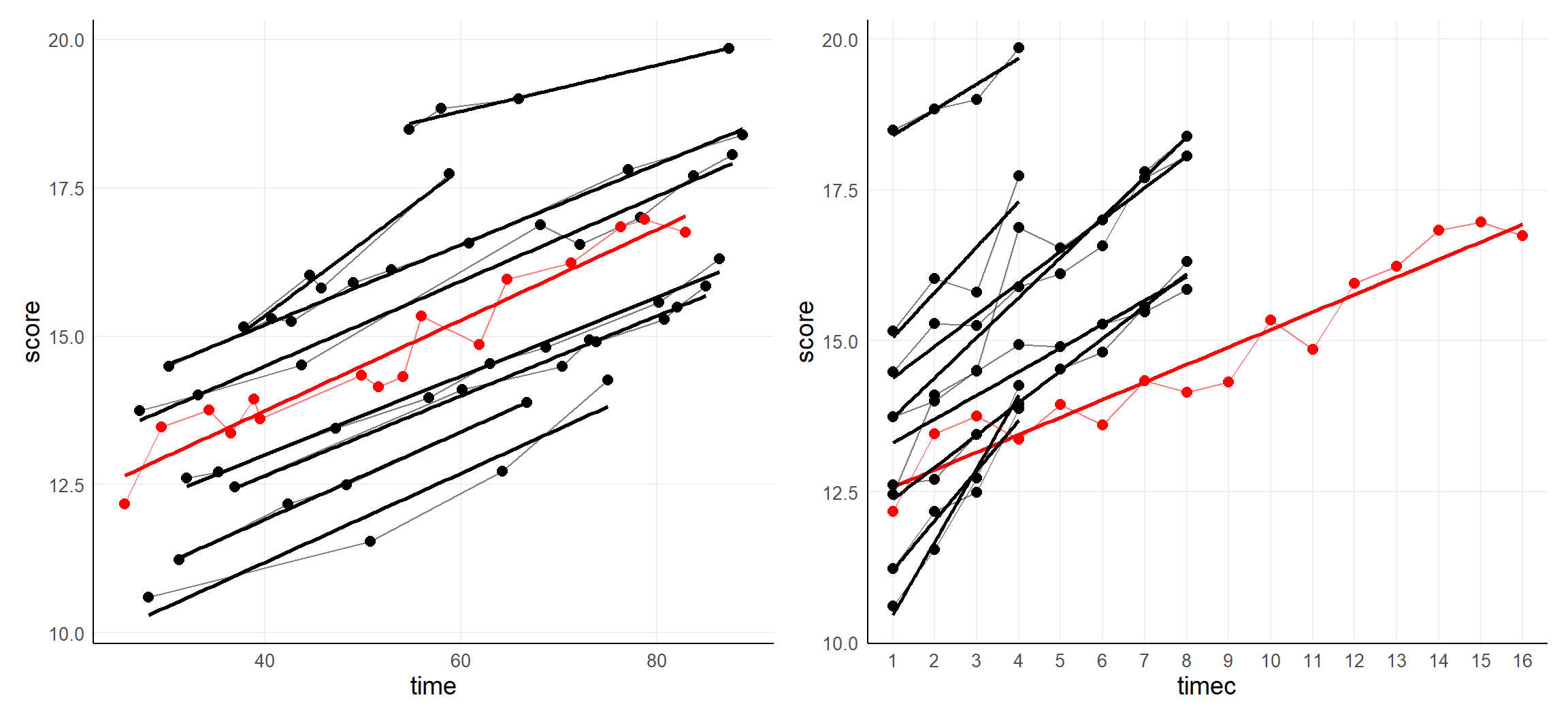
6.1 Categorical and Continuous Time Scale

Time within mixed models

does not require
- equidistance
- fixed timepoints
can be categorical (ordinal) or continuous (numeric)

Choose continuous when:

time is meaningful numerically; time elapsed is a driver
trajectories behave smooth over time

Choose categorical when:

time is not fully meaningful numerically
- order can be a driver
- trajectories change in nature (data generating process)
- e.g., pre-post, 3m, 6m, 12m

Figure 19: Time Scales: Continuous vs Categorical

6.2 The Longitudinal Random Intercept Model

The simplest longitudinal model

individuals start at different baselines
change at the same average rate
just a random intercept model with time as predictor
correlation within clusters, independent of time difference

\[ y_{it} = \underbrace{(\gamma_{00} + u_{0i})}_{\text{person-specific intercept}} + \underline{\gamma_{10} \cdot \text{time}_{it}} + \varepsilon_{it} \]

with: \[ u_{0i} \sim \mathcal{N}(0,\ \tau_{00}), \qquad \varepsilon_{it} \sim \mathcal{N}(0,\ \sigma^2) \]

The model fit now uses time as fixed variable to capture the average change,
while accomodating a constant covariance between residuals remaining.

lmert_int_9 <- lmer(score ~ time + (1 | group), data = dta_timed_x)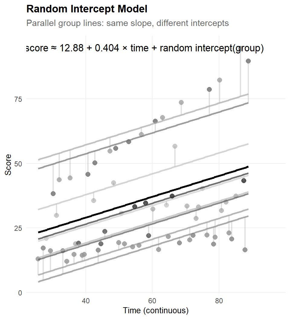

6.2.1 Categorical Time

With 4 time points (T0, T3, T6, T9), we can compare scores in two ways:

Consecutive timepoints: T3 vs T0, T6 vs T3, T9 vs T6 (differences between adjacent times)
All vs reference: T3 vs T0, T6 vs T0, T9 vs T0 (all times compared to baseline)

Expected marginal means used to extract contrasts from a fitted model:

All vs Reference (T0)

Consecutive Comparisons

All Pairwise Comparisons

|  contrast estimate    SE df t.ratio p.value
|  T0 - T3    -0.799 0.245 24  -3.254  0.0166
|  T0 - T6    -1.170 0.245 24  -4.764  0.0004
|  T0 - T9    -2.201 0.245 24  -8.964  <.0001
|  T3 - T6    -0.371 0.245 24  -1.510  0.4475
|  T3 - T9    -1.402 0.245 24  -5.710  <.0001
|  T6 - T9    -1.031 0.245 24  -4.200  0.0017
| 
| Degrees-of-freedom method: kenward-roger 
| P value adjustment: tukey method for comparing a family of 4 estimates

Custom Comparisons can address specific research questions,
E.g., T9 vs avg(T3, T6) uses contrast parameters 0, -0.5, -0.5, 1

|  contrast       estimate    SE df t.ratio p.value
|  T9 - (T6+T3)/2     1.22 0.213 24   5.722  <.0001
| 
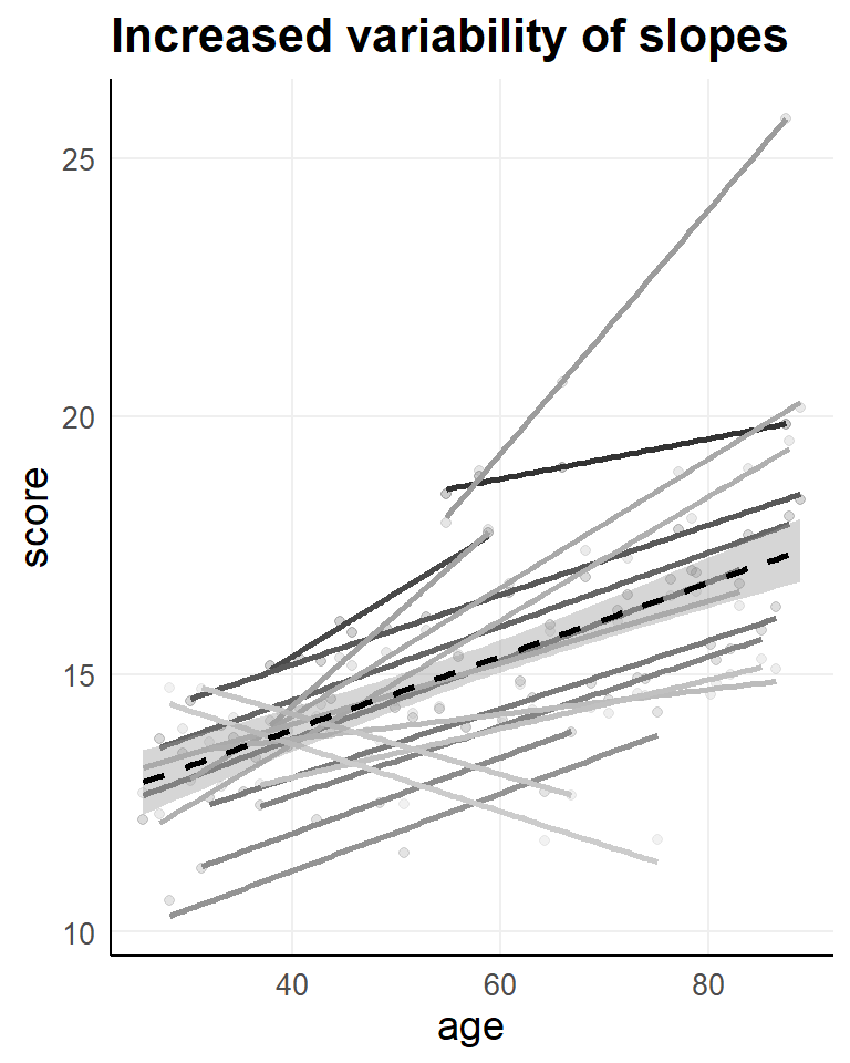
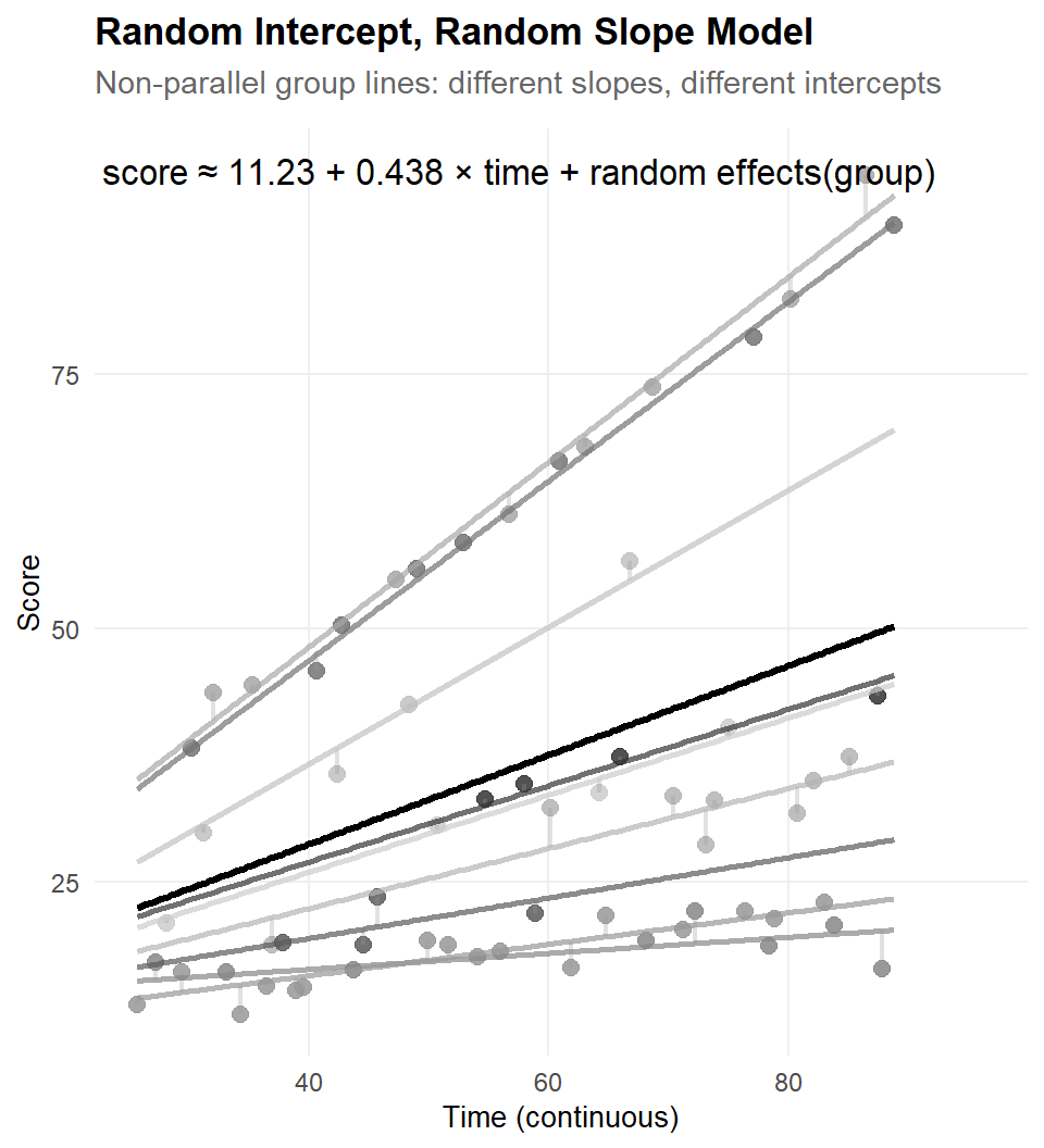
| Degrees-of-freedom method: kenward-roger

6.3 The Longitudinal Random Intercept - Random Slope Model

Heterogeneity can exist over intercept, but also over slopes

individuals differ in slope
with an average slope, and an individual specific difference from that average
time as fixed and random effect

For longitudinal data, individuals can differ in their average but also in their change over time.

\[ y_{it} = (\gamma_{00} + u_{0i}) + (\gamma_{10} + u_{1i}) * \text{time}_{it} + \varepsilon_{it} \]

with: \[ \begin{pmatrix} u_{0i} \\ u_{1i} \end{pmatrix} \sim \mathcal{N}\!\left(\mathbf{0},\ \begin{pmatrix} \tau_{00} & \tau_{01} \\ \tau_{01} & \tau_{11} \end{pmatrix}\right), \qquad \varepsilon_{it} \sim \mathcal{N}(0,\ \sigma^2) \]

The covariance \(\tau_{01}\) is often negative, starting higher results in stronger decrease, or starting lower in stronger increase.

Again: To avoid convergence issues you should center the random slope to reduce colinearity with the intercept.

lmert_slp_9 <- lmer(score ~ time + (1 + time | group), data = dta_timed_x)

effect	group	Term	Estimate	Std. Error	t value	df	p value
fixed	NA	(Intercept)	11.227	1.142	9.830	6.740124	3.07 × 10⁻⁵
fixed	NA	time	0.438	0.105	4.171	8.078695	3.05 × 10⁻³
ran_pars	group	sd__(Intercept)	2.005	NA	NA	NA	NA
ran_pars	group	cor__(Intercept).time	−0.125	NA	NA	NA	NA
ran_pars	group	sd__time	0.312	NA	NA	NA	NA
ran_pars	Residual	sd__Observation	1.908	NA	NA	NA	NA

7 Covariance Structures

Whithin cluster correlational structures:

correlation same for all pairs
correlation different for all pairs
correlation structured (in between the above)

Choose covariance structure for the outcome vector \(\mathbf{y}_i\) of patient \(i\).

Note: covariance structures

implied by the variance-covariance estimated
specified as a repeated measures structure (residual covariance).

For \(T = 4\) time points, the covariance matrix \(\boldsymbol{\Sigma}_i\) is 5×5.

7.1 Most Common Structures

7.1.1 Compound Symmetry (CS)

All variances equal; all covariances equal regardless of time lag.

\[ \boldsymbol{\Sigma}_{\text{CS}} = \begin{pmatrix} \sigma^2 & \rho\sigma^2 & \rho\sigma^2 & \rho\sigma^2 \\ \rho\sigma^2 & \sigma^2 & \rho\sigma^2 & \rho\sigma^2 \\ \rho\sigma^2 & \rho\sigma^2 & \sigma^2 & \rho\sigma^2 \\ \rho\sigma^2 & \rho\sigma^2 & \rho\sigma^2 & \sigma^2 \end{pmatrix} \]

This is exactly what a random intercept model implies. Two parameters: \(\sigma^2\) and \(\rho\).

Note: this is often used for clustered data, not necessarily repeated measurements.

7.1.2 Unstructured (UN)

No constraints — every variance and every covariance is estimated freely. For \(T\) time points: \(T(T+1)/2\) parameters. Most flexible, but most expensive in terms of parameters.

\[ \boldsymbol{\Sigma}_{\text{Unstructured}} = \begin{pmatrix} \sigma_1^2 & \sigma_{12} & \sigma_{13} & \sigma_{14} \\ \sigma_{12} & \sigma_2^2 & \sigma_{23} & \sigma_{24} \\ \sigma_{13} & \sigma_{23} & \sigma_3^2 & \sigma_{34} \\ \sigma_{14} & \sigma_{24} & \sigma_{34} & \sigma_4^2 \end{pmatrix} \]

7.1.3 Heterogeneous Compound Symmetry (CSH)

Like CS, but allows variances to differ across time points. Useful when variability grows over follow-up.

\[ \boldsymbol{\Sigma}_{\text{CSH}} = \begin{pmatrix} \sigma_1^2 & \rho\,\sigma_1\sigma_2 & \rho\,\sigma_1\sigma_3 & \rho\,\sigma_1\sigma_4 \\ \rho\,\sigma_1\sigma_2 & \sigma_2^2 & \rho\,\sigma_2\sigma_3 & \rho\,\sigma_2\sigma_4 \\ \rho\,\sigma_1\sigma_3 & \rho\,\sigma_2\sigma_3 & \sigma_3^2 & \rho\,\sigma_3\sigma_4 \\ \rho\,\sigma_1\sigma_4 & \rho\,\sigma_2\sigma_4 & \rho\,\sigma_3\sigma_4 & \sigma_4^2 \end{pmatrix} \]

7.1.4 Autoregressive Order 1 — AR(1)

Correlation decays exponentially with lag: \(\text{Corr}(y_t, y_{t+k}) = \rho^k\).

\[ \boldsymbol{\Sigma}_{\text{AR(1)}} = \sigma^2 \begin{pmatrix} 1 & \rho & \rho^2 & \rho^3 \\ \rho & 1 & \rho & \rho^2 \\ \rho^2 & \rho & 1 & \rho \\ \rho^3 & \rho^2 & \rho & 1 \end{pmatrix} \]

Two parameters: \(\sigma^2\) and \(\rho\). Natural for equally-spaced measurements with decaying memory.

7.1.5 Heterogeneous AR(1)

Allow the variances to change over time.

\[ \boldsymbol{\Sigma}_{\text{ARH(1)}} = \begin{pmatrix} \sigma_1^2 & \rho\,\sigma_1\sigma_2 & \rho^2\,\sigma_1\sigma_3 & \rho^3\,\sigma_1\sigma_4 \\ \rho\,\sigma_1\sigma_2 & \sigma_2^2 & \rho\,\sigma_2\sigma_3 & \rho^2\,\sigma_2\sigma_4 \\ \rho^2\,\sigma_1\sigma_3 & \rho\,\sigma_2\sigma_3 & \sigma_3^2 & \rho\,\sigma_3\sigma_4 \\ \rho^3\,\sigma_1\sigma_4 & \rho^2\,\sigma_2\sigma_4 & \rho\,\sigma_3\sigma_4 & \sigma_4^2 \end{pmatrix} \]

7.1.6 Toeplitz

Correlations depend only on the lag, but without the exponential constraint of AR(1). Each lag distance has its own parameter. More flexible than AR(1), fewer parameters than unstructured.

\[ \boldsymbol{\Sigma}_{\text{Toeplitz}} = \begin{pmatrix} \tau_0 & \tau_1 & \tau_2 & \tau_3 \\ \tau_1 & \tau_0 & \tau_1 & \tau_2 \\ \tau_2 & \tau_1 & \tau_0 & \tau_1 \\ \tau_3 & \tau_2 & \tau_1 & \tau_0 \end{pmatrix} \]

7.1.7 6. …

Various others exist, choose

most efficient
captures the assumed process
- continuous or not, equidistant or not ?
is in line with the data
- choose based on AIC or BIC (fitted with ML)

8 Effect sizes in mixed models

8.1 Effect size for fuxed effects (random effects and residual variance)

The effect size of a single fixed effect is typically a local effect size similar to Cohen’s \(f^2\), obtained through model comparison (full model vs. reduced model), while keeping the random-effects structure the same.

For a predictor \(b\), one common approximation is

\[ f_b^2 = \frac{R^2_{ab} - R^2_a}{1 - R^2_{ab}}, \]

with \(R^2_{ab}\), proportion of variance explained by the full model,
and \(R^2_a\), proportion explained by the reduced model without predictor \(b\).

This can be approximated using the residual variances:

\[ R^2 = \frac{V_{\text{null}} - V_{\text{model}}}{V_{\text{null}}}. \]

Effect sizes for mixed models are still debated:

Multiple variance components, a single “total” variance is not uniquely defined, resulting in different \(R^2\) definitions
- Marginal \(R^2\): variance explained by fixed effects only, relative to total variance (fixed + all random + residual).
- Conditional \(R^2\): variance explained by fixed + random effects together.
Dependence on random-effects structure, size depends on random-effects structure (e.g., adding random slopes, changing correlation structures), thus hard to compare.
Partial pooling and shrinkage, blurring the boundary between “fixed” and “random”.
Context-specific interpretation, interpretation level specific.

8.2 Effect size for variance estimates (random effects and residual variance)

The effect size for variance parameters is typically expressed as proportions of variance or standardized differences, rather than Cohen’s \(f^2\).

Proportion of total variance attributable to a random effect

\[ \text{ICC} = \frac{\tau_0^2}{\tau_0^2 + \sigma^2}. \]

For more complex models with multiple random components, analogous proportions can be computed, e.g.:

\[ \text{Prop}_{\text{intercept}} = \frac{\tau_0^2}{\tau_0^2 + \tau_{1}^2 + \sigma^2}, \quad \text{Prop}_{\text{residual}} = \frac{\sigma^2}{\tau_0^2 + \tau_{1}^2 + \sigma^2}, \]

with \(\tau_{1}^2\) a random-slope variance
Change in variance components
Comparing models, relative change in a variance component:

\[ \text{RelChange}_{\tau} = \frac{\tau_{\text{null}}^2 - \tau_{\text{model}}^2}{\tau_{\text{null}}^2}, \]

interpreted as the proportion of that random-effect variance “explained” or reduced by the added predictor.
Standardized variance differences
difference in standard deviations between two conditions or models, scaled by a reference standard deviation. For example, treatment changes random-intercept variance from \(\tau_0^2\) to \(\tau_1^2\):

\[ d_{\tau} = \frac{\sqrt{\tau_1^2} - \sqrt{\tau_0^2}}{\sigma_{\text{ref}}}, \]

where \(\sigma_{\text{ref}}\) is a reference residual or total standard deviation.

9 Final Remarks

Mixed models

are regression models, extended with a model for dependencies
explicitly model two (or more) sources of variation:
- within-cluster variation
- between-cluster variation
use clusters (e.g., patients, hospitals, sites), linked through a common population of clusters
capture cluster-specificities through:
- random effects (cluster-specific deviations)
- induced correlation structures for repeated/linked measurements
allow borrowing strength across clusters via partial pooling
provide flexible covariance structures for errors / random effects
- e.g., AR(1), heterogeneous AR(1), compound symmetry, heterogeneous CS, unstructured, Toeplitz
yield more accurate inference for:
- fixed effects (regression coefficients)
- predicted cluster-specific trajectories / means
handle unbalanced data and missing observations naturally
are appropriate for:
- repeated measures, longitudinal data
- hierarchical / nested data
- clustered survey data, multi-site studies

welcome to discuss further @ SQUARE book an appointment through square.research.vub.be