gpower

class: inverse, bottom, left
background-image: url(data:image/png;base64,#assets/images/fish.jpg)
background-size: cover

# Sample Size Calculation with GPower

### in-house workshop
 
.myname[Wilfried @ SQUARE square.research.vub.be April 02, 2023]

<div>
<style type="text/css">.xaringan-extra-logo {
width: 110px;
height: 128px;
z-index: 0;
background-image: url(assets/images/square_logo_margin_blank.png);
background-size: contain;
background-repeat: no-repeat;
position: absolute;
top:0em;right:1em;
}
</style>
<script>(function () {
 let tries = 0
 function addLogo () {
 if (typeof slideshow === 'undefined') {
 tries += 1
 if (tries < 10) {
 setTimeout(addLogo, 100)
 }
 } else {
 document.querySelectorAll('.remark-slide-content:not(.title-slide):not(.inverse):not(.hide_logo)')
 .forEach(function (slide) {
 const logo = document.createElement('div')
 logo.classList = 'xaringan-extra-logo'
 logo.href = null
 slide.appendChild(logo)
 })
 }
 }
 document.addEventListener('DOMContentLoaded', addLogo)
})()</script>
</div>

---
name: context

## Sample Size Calculation with GPower

- Goal
	- to introduce key ideas
	- to offer a perspective for reasoning
	- to offer first practical experience

- Target audience
	- primarily the research community at VUB / UZ Brussel

- Feedback
	- help us improve this document wilfried.cools@vub.be

???
1 + 1:30
introduce researchers to key ideas (know how), 
to help you reason about it (why), 
and make sure you are able to (get it done)

---
name: program

## Program

.pull-left[

- Part I: understand the reasoning
	- introduce building blocks
	- implement on t-test

- Part II: explore more complex situations
	- beyond the t-test
	- simple but common

- GPower
	- not one formula for all
	- a few exercises

]

???
1:30

first focus on essence with simple example
then extend and exercise

---
name: demarcation

## Sample size calculation: demarcation

- How many observations will be sufficient ?
	- avoid too many, because typically observations imply a cost
		- money / time → limited resources
		- risk / harm → ethical constraints
	- depends on the aim of the study
		- research aim &rarr; statistical inference

- Linked to statistical inference (using standard error)
	- testing → power [probability to detect effect]
	- estimation → accuracy [size of confidence interval]

???
5:00 if going slow

It is about answering your research question while avoiding avoidable costs,
only works when focused on inference because of the standard error

---
name: design

## Sample size calculation: a difficult design issue

- Before data collection, during design of study
	- requires understanding: what is a relevant outcome ?!
	- requires understanding: future data, analysis, inference (effect size, focus, ...)
	- decision based on (highly) incomplete information, based on (strong) assumptions

- Not always possible nor meaningful !
	- easier for confirmatory studies, much less for exploratory studies
	- easier for experiments (control), less for observational studies
	- not possible for predictive models, because no standard error
	- NO retrospective power analyses &rarr; OK for future study only
	 
	Hoenig, J., & Heisey, D. (2001). The Abuse of Power: The Pervasive Fallacy of Power Calculations for Data Analysis. The American Statistician, 55, 19–24.

- Alternative justifications often more realistic: 
	- common practice, feasibility, ... or a change of research aim (description, pilot, ...)
	- less strong, puts more weight on non-statistical justification (importance, low cost, ...)

???
8:00

What do you want !?!! because about how to ensure you get it !
And what will the data look like, in practice, not easy because unknown, voodoo
Maybe not always so important because maybe often it is not possible nor meaningful
Then focus on what you can do... explain, convince
Show you have given it careful thought

---
name: example

## Simple example confirmatory experiment

- Example: does this method work for reducing tumor size ?

- evaluation of radiotherapy to reduce a tumor in mice

- comparing treatment group with control (=conditions)
		- tumor induced, random assignment treatment or control (equal if no effect)	
		- after 20 days, measurement of tumor size (=observations)
		- happy if 20% more reduction in treatment !! (=minimal clinically relevant difference)

- intended analysis: unpaired t-test to compare averages for treatment and control

- SAMPLE SIZE CALCULATION:
		- IF average tumor size for treatment at least 20% less than control (4 vs. 5 mm)
		- THEN how many observations sufficient to detect that difference (significance) ?

???
2:00

Just a first possible example where all is straightforward.
It considers the goal, the statistical test.

---
name: reference

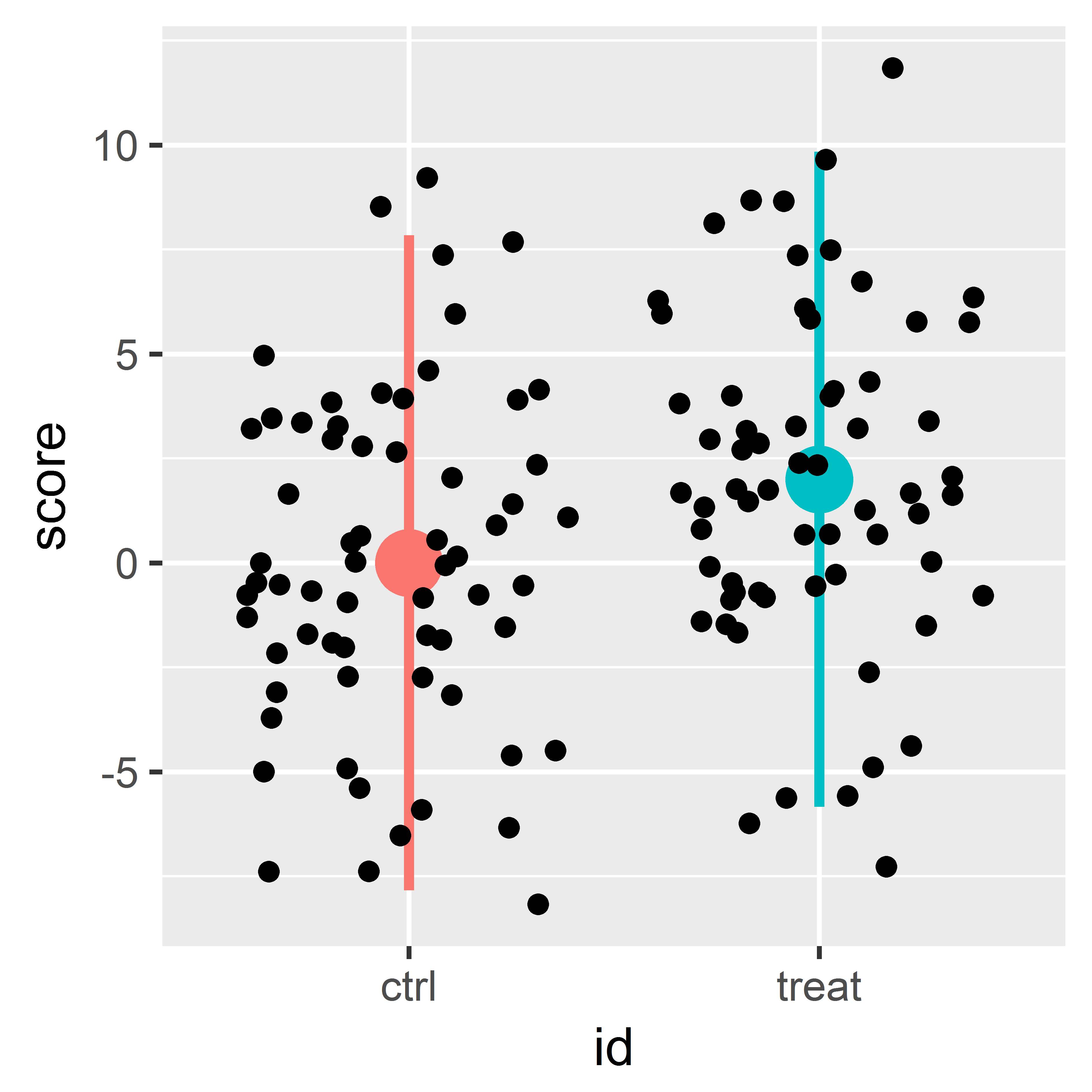
## Reference example

- Reference example used throughout the workshop !!

.pull-left-60[
- Apriori specifications
	- intend to perform a statistical test
	- comparing 2 equally sized groups
	- to detect difference of at least 2
	- assuming an uncertainty of 4 SD on each mean
	- which results in an effect size of .5
	- evaluated on a Student t-distribution
	- allowing for a type I error prob. of .05 `$(\alpha)$`
	- allowing for a type II error prob. of .2 `$(\beta)$`

- Sample size conditional on specifications being true
]
.pull-right-40[
 
<img src="assets/images/ttestData.png" width=300></img>
]

???
2:40

Another example, with values used throughout the workshop. WRITE
delta 2
sigma 4
so effect size .5
alpha .05
beta .2 thus power .8
n ?

---
name: formula

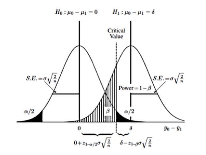
## Formula you could use

.pull-left-60[
- For this particular case:
	- sample size (n &rarr; `?`)
	- difference ( `$\Delta$` =signal &rarr; `2`)
	- uncertainty ( `$\sigma$` =noise &rarr; `4`)
	- type I errors ( `$\alpha$` &rarr; `.05`, so `$Z_{ \alpha /2}$` &rarr; -1.96)
	- type II errors ( `$\beta$` &rarr; `.2`, so `$Z_ \beta$` &rarr; -0.84)

- Sample size = 2 groups x 63 observations = 126

- Note: formula's are test and statistic specific logic remains same

- This and other formula's implemented in various tools our focus: `GPower`
]

.pull-right-40[

`$n = \frac{(Z_{\alpha/2}+Z_\beta)^2 * 2 * \sigma^2}{ \Delta^2}$` 
`$n = \frac{(-1.96-0.84)^2 * 2 * 4^2}{2^2} = 62.79$`

<img src="assets/images/NormalDist.png" width=300></img>
]

???
2:00

It is simple to extract the sample size using only these numbers.
The alpha and beta is interpreted on a normal distribution, as cut-off values for probabilities by quantiles.
This is the simplest case, not the t-distribution which depends on the degrees of freedom.

---
name: block

## GPower: the building blocks in action

.pull-left-70[
- 4 components and 2 distributions
	- distributions: Ho & Ha ~ test dependent shape
	- SIZES: effect size & sample size ~ shift Ha
	- ERRORS : 
		- Type I error ( `$\alpha$` ) defined on distribution Ho
		- Type II error ( `$\beta$` ) evaluated on distribution Ha

- Calculate sample size based on effect size, and type I / II error
]
.pull-right-30[
 
 
<img src="assets/images/gpower_dist.png" width=400></img>
]

???
2:00

One of the distributions reflects the absence of effect, the other combines the size of the effect and the information available to try and detect that effect.
The actual distributions depend on the statistical test of interest.
The shift depends on both; effect size and sample size.
The shift has consequences for how much of the Ha distribution is beyond the cut-off at Ho distribution.
The only issue is how far the distribution shifts...

---
name: gpower

## GPower: a useful tool

.pull-left-60[
- Use it
	- implements wide variety of tests
	- free @ http://www.gpower.hhu.de/
	- popular and well established
	- implements various visualizations
	- documented fairly well

- Maybe not use it
	- not all tests are included !
	- not without flaws !
	- other tools exist (some paying)
	- for complex models: impossible 
		alternative: simulation (generate and analyze)
]
.pull-right-40[
<img src="assets/images/GPowerStart.png" width=100%></img>
]

???
2:30

GPower because it offers calculations for different tests, no need to study formulas.
There are good reasons to use it, but... not all is perfect.

---
name: test

## GPower statistical tests

.pull-left[
- Test family - statistical tests [in window]
	- Exact Tests (8)
	- `$t$`-tests (11) &rarr; `reference`
	- `$z$`-tests (2)
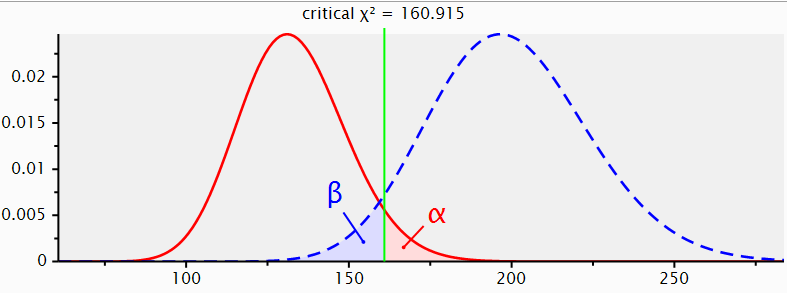
	- `$\chi^2$`-tests (7) 
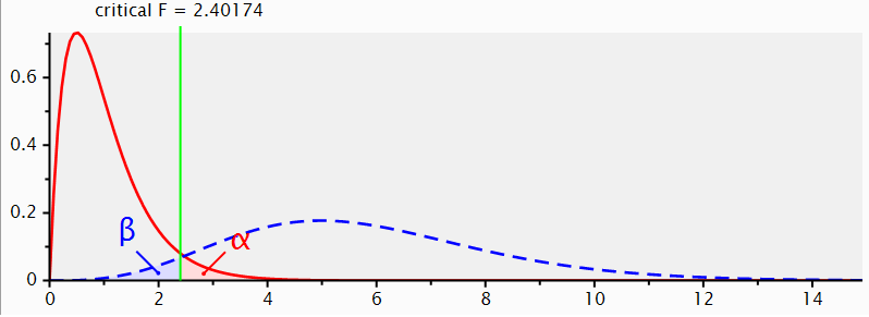
	- `$F$`-tests (16)
- Focus on the density functions
]
.pull-right[
- Tests [in menu]
	- correlation & regression (15)
	- means (19) &rarr; `reference`
	- proportions (8)
	- variances (2)
- Focus on the type of parameters
]
.pull-left[
<img src="assets/images/Xdist.png" width=500></img>
]
.pull-right[
<img src="assets/images/Fdist.png" width=500></img>
]

???
1:30

Before focus on one of the 11 t-test, or one of the 19 means comparisons, however you want to look at it.
Various other tests exist, categorized in one of two ways.

---
name: input

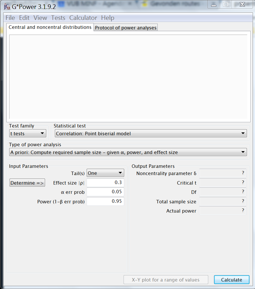
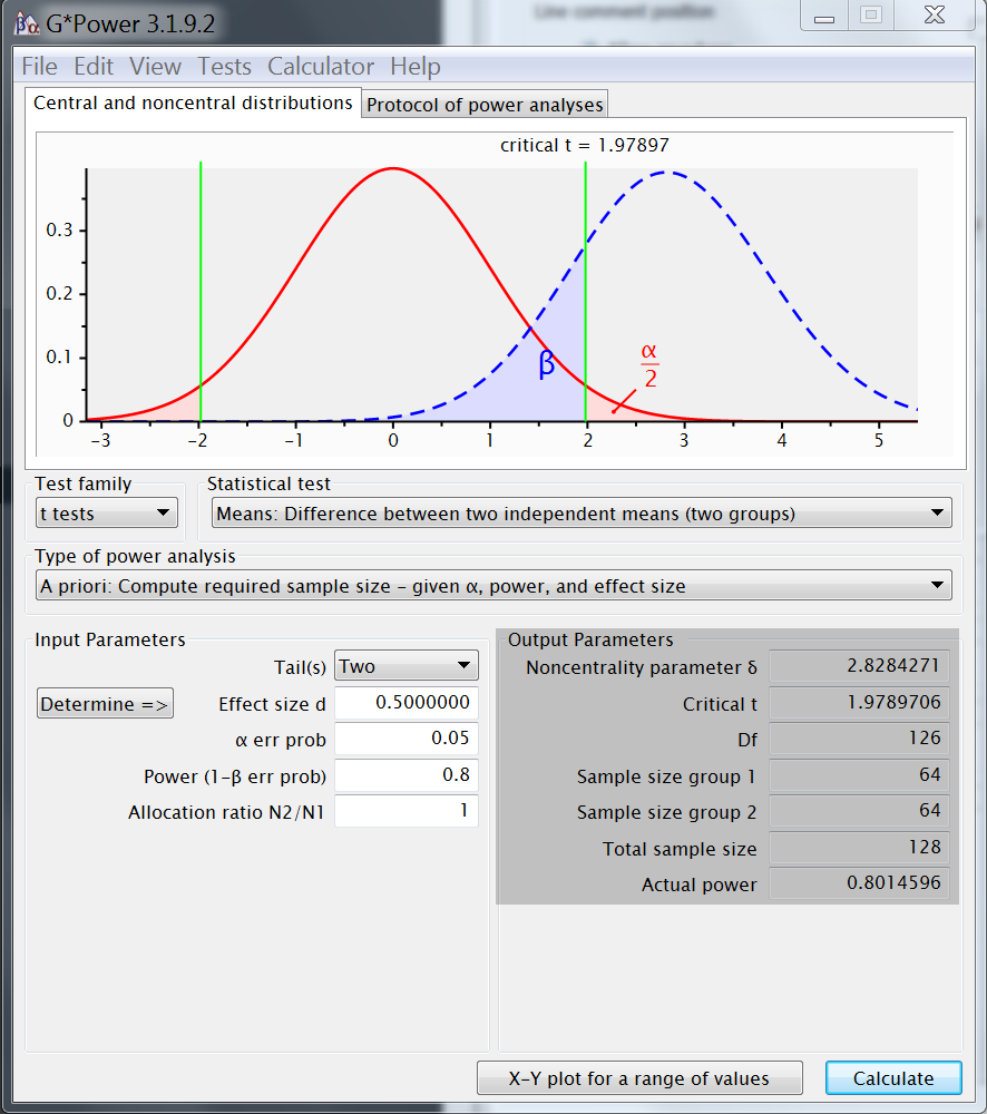
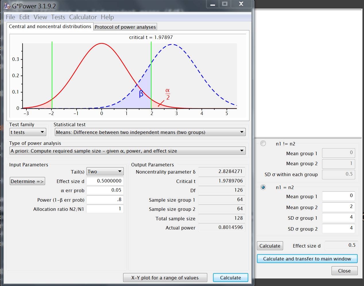
## GPower input

.pull-left[
- `~ reference example input`
	- t-test : difference two indep. means
	- apriori: calculate sample size
	- effect size = standardized difference
		- Cohen's `$d$`
		- Determine =>
		- `$d$` = |difference| / SD_pooled
		- `$d$` = |`0-2`| / `4` = `.5`
	- `$\alpha$` = `.05` 2 - tailed <mini>( `$\alpha$` /2 &rarr; .025 & .975 )</mini>
	- `$power = 1-\beta$` = `.8`
	- allocation ratio N2/N1 = `1` (equally sized groups)
]
.pull-right[
<img src="assets/images/GPowerEx1xInput.png" width=100%></img>
]

???
2:00

For the reference example the input is given, t
effect sizes are specified with 'determine'.

We choose a test, type, 
to get sample size, we use effect size 2/4, alpha .05 and beta .2.

SHOW MARKER

---
name: output

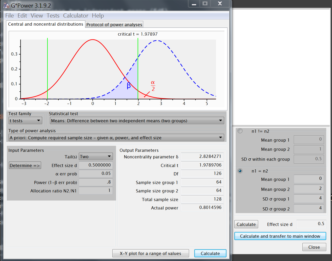
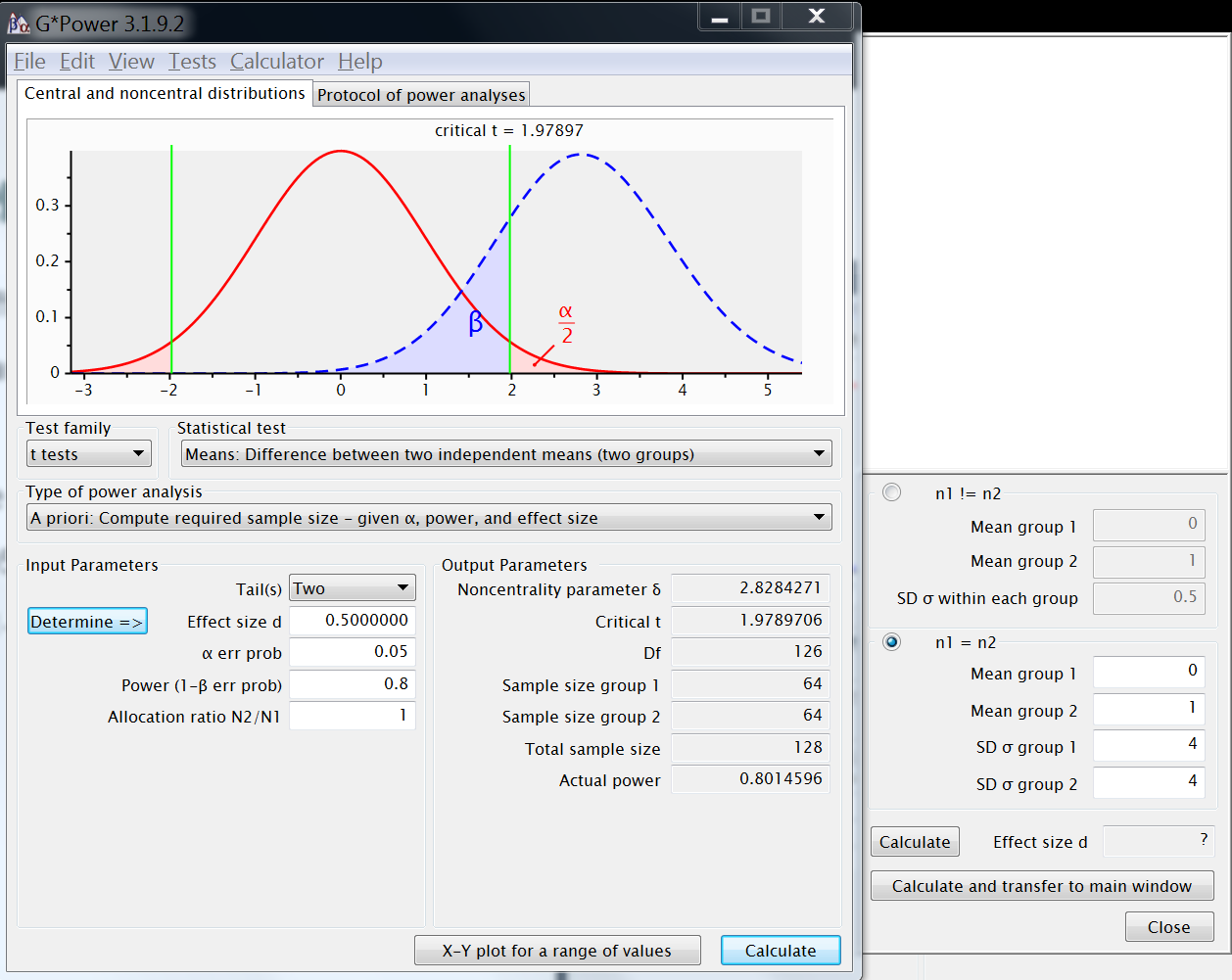
## GPower output

.pull-left[

- `~ reference example output`
	- sample size `$(n)$` = 64 x 2 = (`128`)
	- degrees of freedom `$(df)$` = 126 (128-2)
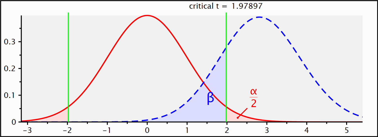
	- critical t = 1.979
		- decision boundary given `$\alpha$` and `$df$` `qt(.975,126)`
	- non centrality parameter ( `$\delta$` ) = 2.8284
		- shift `Ha` (true) away from `Ho` (null) `2/(4*sqrt(2))*sqrt(64)`
	- distributions: central + non-central
	- power &ge; .80 (1- `$\beta$`) = 0.8015
]
.pull-right[
<img src="assets/images/GPower1Output.png"></img>
]

???
2:30

The result is 'almost' the same as before, with the normal distribution, but slightly less efficient.
The critical t depends on the degrees of freedom (or sample size).
The resulting non-centrality parameter (shift) combines effect size and sample size.

SHOW MARKER

---
name: reference

## GPower protocol

- Summary for future reference or communication
- File/Edit save or print file (copy-paste)

t tests - Means: Difference between two independent means (two groups) 
Analysis:	A priori: Compute required sample size

.pull-left[
Input:	 
	Tail(s)	= Two 
	Effect size `d`	= `0.5000000` 
	`α` err prob = `0.05` 
	Power (`1-β` err prob)	= `.8` 
	Allocation ratio N2/N1	= `1` 
]
.pull-right[
Output:	 
	`Noncentrality` parameter δ	= `2.8284271` 
	`Critical t` = `1.9789706` 
	Df = `126` 
	Sample size group 1	= `64` 
	Sample size group 2	= `64` 
	Total `sample size`	= `128` 
	Actual power = `0.8014596` 
]

???
00:30

Maybe convenient is that you can copy-paste the resulting output (and input) into a text file, to communicate to others or yourself later.

---
name: ncp

## Non-centrality parameter ( `$\delta$` ), shift `Ha` from `Ho`

.pull-left-70[
- `Ho` acts as `$\color{red}{benchmark}$` &rarr; eg., no difference
	- set `$\color{green}{cut off}$` on `Ho ~ t(ncp=0,df)` using `$\alpha$`, 
	- reject `Ho` if test returns `implausible` value

- `Ha` acts as `$\color{blue}{truth}$` &rarr; eg., difference of .5 SD
	- `Ha ~ t(ncp!=0,df)`
	- `$\delta$` as violation of `Ho` &rarr; shift (location/shape)

- `$\delta$`, the non-centrality parameter
	- combines
		- assumed `effect size` (target or signal)
		- conditional on `sample size` (information)
	- determines overlap (power &harr; sample size)
		- probability beyond `$\color{green}{cut off}$` at `Ho` evaluated on `Ha`

]
.pull-right-30[
<img src="assets/images/GPower1.png" width=350></img>
]

???
4:00

All depends on the difference between the distribution assuming no effect, and the one representing the effect of interest.
The shift is quantified by the non-centrality parameter, which combines sample and effect size.

---
name: asymmetry

## Note: Ho and Ha, asymmetry in statistical testing

- `Ha` is NOT interchangeable with `Ho`

- Cut-off at `Ho` using `$\alpha$` 
	- in statistics &rarr; observe test statistics (`Ha` unknown)
	- in sample size calculation &rarr; assume `Ha`

- If fail to reject then remain in doubt
	- absence of evidence `$\neq$` evidence of absence 
		- p-value &rarr; P(statistic|`Ho`) != P(`Ho`|statistic)
		- example: evidence for insignificant `$\eta$` same as for `$\eta$` * 2

- Equivalence testing &rarr; `Ha` for 'no effect'
	- reject `Ho` that smaller than 0 - | `$\Delta$` | AND bigger than 0 + | `$\Delta$` |
	- acts as two superiority tests with margin, combined

???
07:00

While simply the difference matters, between Ho and Ha, 
in statistics they are not the interchangeable.
The alternative is just an assumed effect.

---
name: by_N

## Alternative: divide by N

.pull-left-60[
- Constant difference, changing shape
	- divide by n: sample size ~ standard deviation
	- non-centrality parameter: sample size ~ location
<img src="assets/images/BellePowerCurve.png" width=500></img>
]
.pull-right-40[
`$n = \frac{(Z_{\alpha/2}+Z_\beta)^2 * 2 * \sigma^2}{d^2}$` 
`$n = \frac{(-1.96-0.84)^2 * 2 * 4^2}{2^2}$` 
`$n = 62.79$`

]

???
2:30

The non-centrality parameter combines effect and sample size, 
alternatively sample size could be looked at separately.
Here the shape changes with growing sample size.

---
name: error_probs

## Type I/II error probability

.pull-left-70[
- Inference test based on cut-off's  (density &rarr; AUC=1)

- Type I error: incorrectly reject `Ho` (false positive):  
	- cut-off at `Ho`, error prob. `$\alpha$` controlled
	- one/two tailed &rarr; one/both sides informative ?

- Type II error: incorrectly fail to reject `Ho` (false negative):  
	- cut-off at `Ho`, error prob. `$\beta$` obtained from `Ha`
	- `Ha` assumed known in a power analyses

- power = 1 - `$\beta$` = probability correct rejection (true positive)

- Inference versus truth
	- infer: effect exists vs. unsure
	- truth: effect exist vs. does not
]
.pull-right-30[
<img src="assets/images/GPower1.png"></img>
 
<table>
<tr>
<td></td>
<td>infer=Ha</td>
<td>infer=Ho</td>
<td>sum</td>
</tr>
<tr>
<td>truth=Ho</td>
<td> `$\alpha$`</td>
<td>1- `$\alpha$`</td>
<td>1</td>
</tr>
<tr>
<td>truth=Ha</td>
<td>1- `$\beta$` </td>
<td> `$\beta$` </td>
<td>1</td>
</tr>
</table>

]

???
3:00

Inference is based on the cut-off values, and so errors are possible.  
Either it is incorrectly after the cut-off, considered from Ho,
or it is incorrectly before the cut-off.
Moving the cut-off makes one error bigger and the other smaller, 
but not with equal amounts !
Given a 'truth', the probability sums up to one, you are either right or wrong.

---
name: ex_plot_1

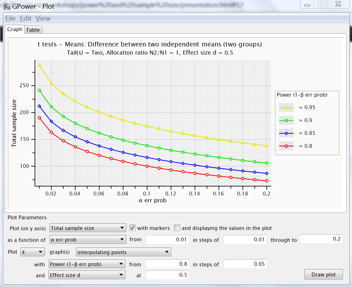
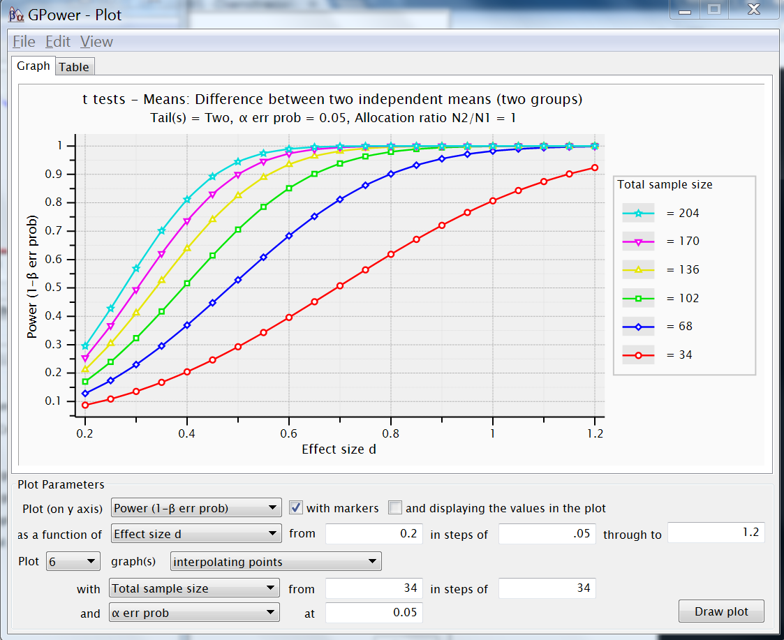
## Create plot

- create plot
	- X-Y plot for range of values
	- Y-axis / X-axis / curves and constant

.pull-left[
- assumes calculated analysis
	- `~ reference example`
- beware of order !
- plot sample size (y-axis)
- by type I error `$\alpha$` (x-axis)
	- from .01 to .2 in steps of .01
- for 4 values of power (curves)
	- with values .8 in steps of .05
- and assume an effect size (constant)
	- .5 from the reference example
]
.pull-right[
- notice Table option
<img src="assets/images/gpErrorEx1.png" width=500></img>
]

???
2:00 + 3:00

order is important
do it yourself after I did

---
name: ex_plot_2

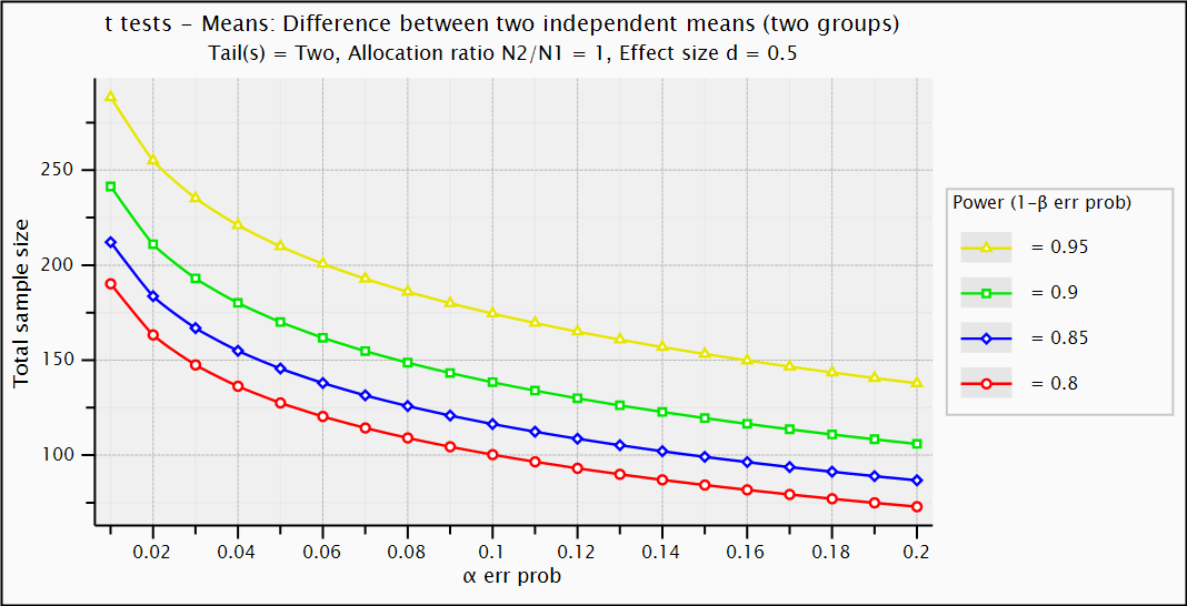
## Exercise on errors, interpret plot

- Understand the building blocks, interpret the plot

.pull-left-60[
- where on the red curve (right) type II error = 4 * type I error ?
- when smaller effect size (.25), what changes ?
- plot power instead of sample size 
	- with 4 power curves with sample sizes 32 in step of 32
	- what is relation type I and II error ?

<img src="assets/images/gpErrorEx2.png" width=70%></img>
]
.pull-right-40[
<img src="assets/images/GPowerPowerError.png"></img>

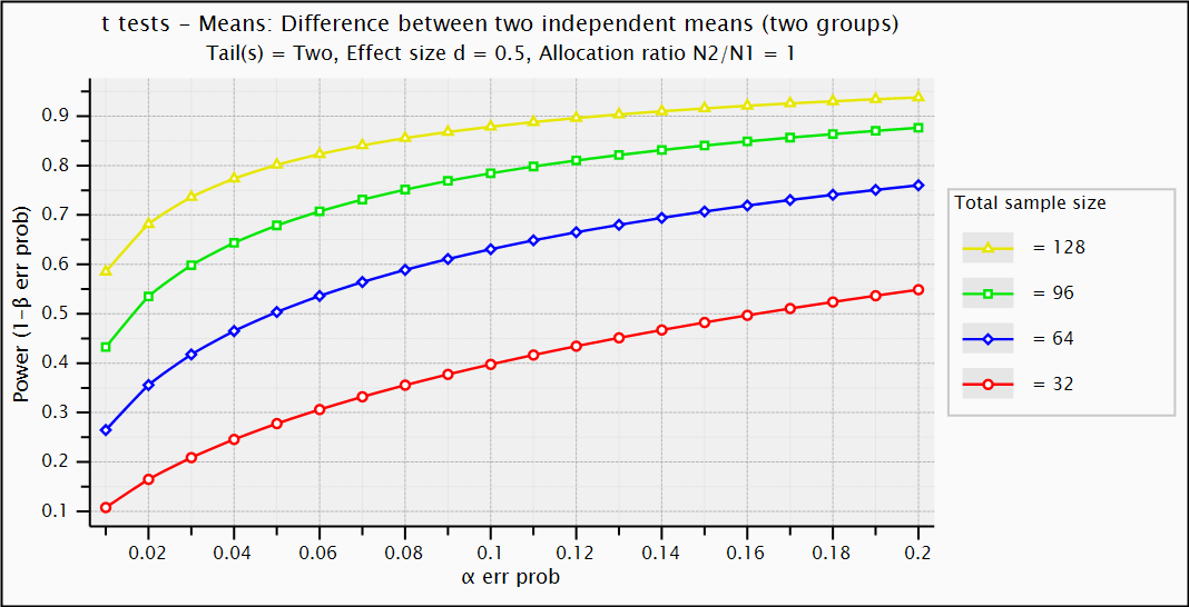
- what would be difference between curves for `$\alpha$` = 0 ?
]

???
1:00 + 3:00

red is power .8, so type II is .2, divided by 4 is .05 for alpha
sample size range changes, change one building block, Y-axis responds, same curves
if type I error up, power up, so II down, given the rest, but not all same strength of change
if you do not allow for any type I, then power is 0, because infinity on t-distribution

---
name: error_decide

## Decide Type I/II error probability

.pull-left-60[
- Popular choices
	- `$\alpha$` often in range .01 - .05 &rarr; 1/100 - 1/20
	- `$\beta$` often in range .2 to .1 &rarr; power = 80% to 90%

- `$\alpha$` & `$\beta$` inversely related
	- power = 1 - `$\beta$` > 1 - 2 * `$\alpha$`
	- `$\alpha$` & `$\beta$` often selected in 1/4 ratio type I error is 4 times worse !!
	- which error you want to avoid most ?
		- cheap aids test ? &rarr; avoid type II
		- heavy cancer treatment ? &rarr; avoid type I
	- probability for errors always exists

]
.pull-right-40[
<img src="assets/images/GPower1.png" width=350></img>
]

???
2:00

popular choices, in ratios / percentages
inversely related, so make a choice
what error you want to avoid most
look at surfaces, .025 * 8 for .2

---
name: error_control

## Control Type I error

- Defined on the Ho, known
	- assumes only sampling variability

- Multiple testing
	- typically used to explore effects in more detail
	- inflates type I error `$\alpha$` (each peak possible error)
	- family of tests: `$1-(1- \alpha)^k$` &rarr; correct, eg., Bonferroni ( `$\alpha/k$`)

- Interim analysis
	- interim analysis (analyze and conditionally proceed)
	- plan in advance
	- alpha spending, eg., O'Brien-Flemming bounds
	- NOT GPower
		- our own simulation tool (Susanne Blotwijk): 
		http://apps.icds.be/simAlphaSpending/
	- determine boundaries with PASS, R (ldbounds), ...

???
5:00 + 1:00

alpha on the Ho, so under control, assumes variation only due to sampling
if multiple tests, each time possible error, prob error at least once increases
compensate for multiple testing, 1 minus each time correct, bonferoni is simple way to get that
with interim, also multiple testing, make decision, not only sampling, account for that
alpha spending, different boundaries with adjusted alphas that total alpha
not in Gpower, have a look at susanne

---
name: fun

## For fun: P(effect exists | test says so)

- Using `$\alpha$`, `$\beta$` and power or `$1-\beta$`
	- `$P(infer=Ha|truth=Ha) = power$` &rarr; `$P$`(test says there is effect | effect exists)
	- `$P(infer=Ha|truth=Ho) = \alpha$`
	- `$P(infer=Ho|truth=Ha) = \beta$`  
	- `$P(\underline{truth}=Ha|\underline{infer}=Ha) = \frac{P(infer=Ha|truth=Ha) * P(truth=Ha)}{P(infer=Ha)}$` &rarr; Bayes Theorem
	- __ = `$\frac{P(infer=Ha|truth=Ha) * P(truth=Ha)}{P(infer=Ha|truth=Ha) * P(truth=Ha) + P(infer=Ha|truth=Ho) * P(truth=Ho)}$`
	- __ = `$\frac{power * P(truth=Ha)}{power * P(truth=Ha) + \alpha * P(truth=Ho)}$` &rarr; depends on prior probabilities

- IF very low probability model is true (eg., .01) &rarr; `$P(truth=Ha) = .01$`
- THEN probability effect exists if test says so is low, in this case only .14 !!
 
- `$P(truth=Ha|infer=Ha) = \frac{.8 * .01}{.8 * .01 + .05 * .99} = .14$`

???
5:00

---
name: size_principle

## Effect sizes, in principle

- Estimate/guestimate of minimal magnitude of interest

- Typically standardized: signal to noise ratio (noise provides scale)
	- eg., effect size `$d$` = .5 means .5 standard deviations
	- eg., difference on scale of pooled standard deviation

- Part of non-centrality (as is sample size) &rarr; pushing away `Ha`

- ~ practical relevance (not statistical significance)
	- NOT p-value ~ partly effect size, but also partly sample size

- 2 main families of effect sizes (test specific)
	- `d-family` (differences) and `r-family` (associations)
	- transform one into other, eg., d = .5 &rarr; r = .243 
	`$\hspace{20 mm}d = \frac{2r}{\sqrt{1-r^2}}$` `$\hspace{20 mm}r = \frac{d}{\sqrt{d^2+4}}$` `$\hspace{20 mm}d = ln(OR) * \frac{\sqrt{3}}{\pi}$`

???
4:00

third building block, effect, magnitude
standardized so that meaningful to interpret and compare
signal to noise ratio, 2/4 = .5, really is .5 standard deviations
means, difference on scale of pooled sd's
while part of non centrality, does not include sample size
statistical significance does include sample size

`$V_d = \frac{4V_r}{(1-r^2)^3}$`; `$\hspace{15 mm}V_r = \frac{4^2V_d}{(d^2+4)^3}$`; `$\hspace{15 mm}V_d = V_{ln(OR)} * \frac{3}{\pi^2}$`

---
name: size_literature

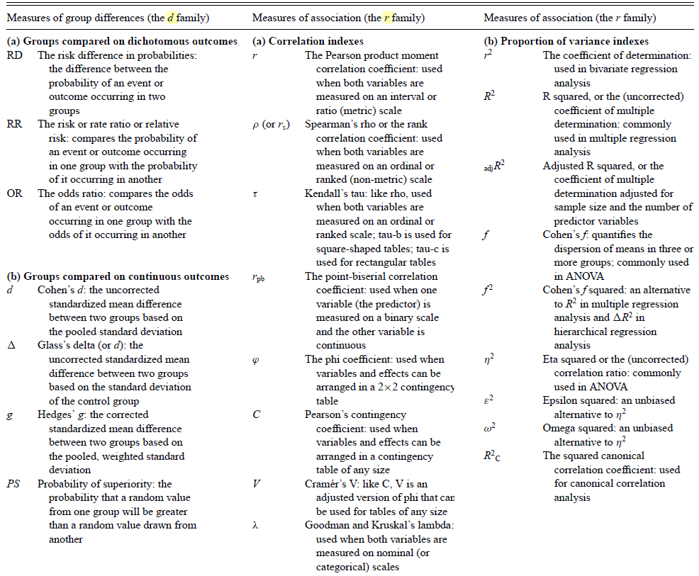
## Effect sizes, in literature

.pull-left-40[
- Cohen, J. (1992). A power primer. Psychological Bulletin, 112, 155–159.

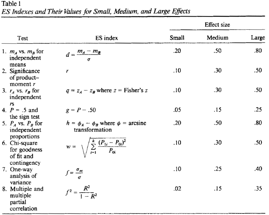
- Cohen, J. (1988). Statistical power analysis for the behavioral sciences (2nd ed). 
- famous Cohen conventions but beware, just rules of thumb
]
.pull-right-60[
- more than 70 different effect sizes... most of them related
- Ellis, P. D. (2010). The essential guide to effect sizes: statistical power, meta-analysis, and the interpretation of research results.
<img src="assets/images/ES2.png" width=70% style="float: right;"></img>
]

???
1:00

---
name: size_determine

## Effect sizes, in GPower (Determine)

.pull-left-60[
- Effect sizes are test specific
	- t-test &rarr; group means and sd's
	- one-way anova &rarr; variance explained & error
	- regression &rarr; sd's and correlations
	- . . . .

- GPower helps with `Determine`
	- sliding window
	- one or more effect size specifications
]
.pull-right-40[
<img src="assets/images/GPowerEx1x.png" width=500></img>
]

???

GPOWER t-f-r-...
the determine button opens a window to help specify the effects size
given certain values, others are calculated
and transferred to the main window

---
name: ex_size

## Exercise on effect sizes, ingredients Cohen's d

.pull-left[
- For the `reference example`: 
	- change mean values from 0 and 2 to 4 and 6, what changes ?
	- change sd values to 2 for each, what changes ?
		- effect size ?
		- total sample size ?
		- critical t ?	
		- non-centrality ? 
	- change sd values to 8 for each, what changes ? 
	- change sd to 2 and 5.3, or 1 and 5.5, how does it compare to 4 and 4 ? 
]
.pull-right[
<img src="assets/images/GPower0.png" width=500></img>
]

???
d = standardized difference
less noise, better signal to noise ratio
effect size bigger, less sample size THUS slightly larger t cut off
no clear relation with ncp because effect size + sample size -
more noise, opposite
with difference in sd, bigger has more impact, much lower compensates a bit higher

---
name: ex_size_plot

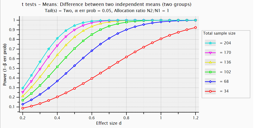
## Exercise on effect sizes, plot

.pull-left[
- For the `reference example`: 
	- plot powercurve: power by effect size
	- compare 6 sample sizes: 34 in steps of 34
	- for a range of effect sizes in between .2 and 1.2
	- use `$\alpha$` equal to .05
	 
	- pinpoint the situations from previous section on the plot (sd=4 and 2).
	- how does power change when doubling the effect size ?
]
.pull-right[
- powercurve &rarr; X-Y plot for range of values
 
<img src="assets/images/GPowerPowerESx.png" width=500></img>
]

???

power by effect size, beware of changes after including the 6 power curves
effect sizes .2 to 1.2, in steps of whatever, maybe .1
the sd 4 situation, comes with 64 observations, blue, effect size .5
the sd 2, is effect size 1 on 34, red
doubling the effect size shows increase in power, but not for all the same

---
name: ex_imbalance

## Exercise on effect size, imbalance

.pull-left[
- For the `reference example`:
	- compare for allocation ratios 1, .5, 2, 10, 50
	- repeat for effect size 1, and compare

- ? no idea why n1 `$\neq$` n2 
<img src="assets/images/GPower0.png" width=300></img>
]
.pull-right[
<img src="assets/images/GPowerPowerES.png" width=500></img>

after calculate plot, 
to change allocation ratio
]

???
allocation of /2 or *2 is same, just largest group differs, and can differ if standard deviations differ
but does not show, so, maybe not OK
effect size does not influence the increase much (multiplication)

2	10	18	28	50
38	98	160	238	412
144	382	632	955	1638

---
name: size_specify

## Effect sizes, how to determine them in theory

- Choice of effect size matters &rarr; justify choice !!

- Choice of effect size depends on aim of the study
	- realistic (eg., previously observed effect) &rarr; replicate
	- important (eg., minimally relevant effect)
	- NOT significant &rarr; meaningless, dependent on sample size

- Choice of effect size dependent on statistical test of interest
	- for independent t-test &rarr; means and standard deviations
	- possible alternative: variance explained, eg., 1 versus 16+1
		- with one-way ANOVA ( `$f$` = .25 instead of d = .5)
		- with linear regression ( `$f^2$` = .0625 instead of d = .5)
		- https://www.psychometrica.de/effect_size.html#transform

???
the most important is importance, if you know what matters, you can power your study to detect that
usually just go to literature, find what already found, ensures realistic values, but not necessarily relevant ones
never use significance itself, it is meaningless, it depends on sample size and is therefore not an effect size.

also here, one effect size can be transformed into the next, d to f, to f2
many more transformations at psychometrica

---
name: size_practice

## Effect sizes, how to determine them in practice

- Experts / patients &rarr; use if possible &rarr; importance minimally clinically relevant effect

- Literature (earlier study / systematic review) &rarr; beware of publication bias &rarr; realistic

- Pilot &rarr; guestimate dispersion estimate (not effect size &rarr; small sample)

- Internal pilot &rarr; conditional power (sequential)

- Guestimate uncertainty...
	- sd from assumed range, assume normal and divide by 6
	- sd for proportions at conservative .5
	- sd from control, assume treatment the same
	- `...`

- Turn to Cohen &rarr; use if everything else fails (rules of thumb)
	- eg., .2 - .5 - .8 for Cohen's d

???

easier said than done, often it is and remains difficult
you can ask experts or patients even, for example to get a pain threshold
literature, ok, if it is relevant, but maybe a bit over optimistic
a pilot can help to get an idea of the dispersion, not the effect because too few data
an internal pilot is possible, maybe get an estimate of the sd along the way to re-calibrate
or just try your best to guess, maybe from an assumed range ?
avoid rules of thumb of cohen

---
name: blocks_relation

## Relation sample & effect size, type I & II errors

.pull-left[
- Building blocks: 
	- sample size ( `$n$` )
	- effect size ( `$\Delta$` )
	- alpha ( `$\alpha$` )
	- power ( `$1-\beta$` )

- each parameterconditional on others
]
.pull-right[
- GPower &rarr; type of power analysis
	- Apriori: `$n$` `~` `$\alpha$`, `power`, `$\Delta$`
	- Post Hoc: `power` `~` `$\alpha$`, `$n$`, `$\Delta$` 
	- Compromise: `power`, `$\alpha$` `~` `$\beta\:/\:\alpha$`, `$\Delta$`, `$n$`
	- Criterion: `$\alpha$` `~` `power`, `$\Delta$`, `$n$`
	- Sensitivity: `$\Delta$` `~` `$\alpha$`, `power`, `$n$`

<img src="assets/images/flow.gif" width=500></img>
]

???

All four building blocks combined, and one obtained based on the others.
So far, worked with apriori, to get the sample size.
But also popular, to get the power, then you need alpha, n and delta, (post hoc) OR the relation between alpha and beta (compromise)
Not sure why you would extract alpha, this is typically under control
but you could use delta, often done, but maybe not always ok, see what effect size is possible with the available data.

---
name: ex_type

## Exercise on type of power analysis

- For the `reference example`:
	- retrieve power given n, `$\alpha$` and `$\Delta$`
	- then, for power .8, take half the sample size, how does `$\Delta$` change ? 
	- then, set `$\beta$`/ `$\alpha$` ratio to 4, what is `$\alpha$` & `$\beta$` ? what is the critical value ? 
	- then, keep `$\beta$`/ `$\alpha$` ratio to 4 for effect size .7, what is `$\alpha$` & `$\beta$` ? critical value ?

???

power for the reference was .8, we find it as such
with half the size of sample, the effect size goes up a bit .5 to .7714
when using a ratio, it is .1 and .4, or .05 and .2,

- use post-hoc 64x2 &rarr; .8
- then, for power .8, take half the sample size, how does `$\Delta$` change ? 
	- use sensitivity 32x2 (d=.7114)
	- `$\Delta$` from .5 to .7115 = .2115
	- bigger effect `$\Delta$` compensates loss of sample size n
- then, set `$\beta$` / `$\alpha$` ratio to 4, what is `$\alpha$` & `$\beta$` ? what is the critical value ? 
	- use compromise 32x2
	- `$\alpha$` =.09 and `$\beta$` =.38, critical value 1.6994
- then, keep `$\beta$` / `$\alpha$` ratio to 4 for effect size .7
	- use compromise 32x2
	- `$\alpha$` =.05 and `$\beta$` =.2, critical value 1.9990

---
name: ex_type_solution
exclude: false

## Solution for type of power analysis

- For the `reference example`:
	- retrieve power given n, `$\alpha$` and `$\Delta$`	of `reference` case
		- use post-hoc 64x2 &rarr; .8
	- then, for power .8, take half the sample size, how does `$\Delta$` change ? 
		- use sensitivity 32x2 (d=.7114)
		- `$\Delta$` from .5 to .7115 = .2115
		- bigger effect `$\Delta$` compensates loss of sample size n
	- then, set `$\beta$` / `$\alpha$` ratio to 4, what is `$\alpha$` & `$\beta$` ? what is the critical value ? 
		- use compromise 32x2
		- `$\alpha$` =.09 and `$\beta$` =.38, critical value 1.6994
	- then, keep `$\beta$` / `$\alpha$` ratio to 4 for effect size .7
		- use compromise 32x2
		- `$\alpha$` =.05 and `$\beta$` =.2, critical value 1.9990

???

---
name: gpower_calculator

## Getting your hands dirty

.pull-left[
<img src="assets/images/GPower1.png" width=200></img>

`# calculator`  
`m1=0;m2=2;s1=4;s2=4`  
`alpha=.025;N=128`  
`var=.5*s1^2+.5*s2^2`  
`d=abs(m1-m2)/sqrt(2*var)*sqrt(N/2)`  
`tc=tinv(1-alpha,N-1)`  
`power=1-nctcdf(tc,N-1,d)`  
]

.pull-right[

- in `R`
	- qt &rarr; get quantile on `Ho` ( `$Z_{1-\alpha/2}$` )
	- pt &rarr; get probability on `Ha` (non-central)

```r
.n <- 64
.df <- 2*.n-2
.ncp <- 2 / (4 * sqrt(2)) * sqrt(.n)
.power <- 1 -
	pt(
		qt(.975,df=.df),
		df=.df,	ncp=.ncp
	) - 
	pt( qt(.025,df=.df), df=.df, ncp=.ncp)
round(.power,4)
```

```
## [1] 0.8015
```
]

???

You can calculate in Gpower, but, why would you do that.
In R, get the cutoff on Ho, get probability on Ha, simple
The two sided, has one side almost 0

---
name: beyond-t

## GPower, beyond the independent t-test

- So far, comparing two independent means

- From now on, selected topics beyond independent t-test with small exercises
	- dependent instead of independent
	- non-parametric instead of assuming normality
	- relations instead of groups (regression)
	- correlations
	- proportions, dependent and independent
	- more than 2 groups (compare jointly, pairwise, focused)
	- more than 1 predictor
	- repeated measures

- Look into <a href="http://www.gpower.hhu.de/fileadmin/redaktion/Fakultaeten/Mathematisch-Naturwissenschaftliche_Fakultaet/Psychologie/AAP/gpower/GPowerManual.pdf" target="_new">GPower manual</a> 27 tests &rarr; effect size, non-centrality parameter and example !!

???

---
name: dependence

##  Dependence between groups

- If 2 dependent groups (eg., before/after treatment) &rarr; account for correlations

- Correlation typically obtained from pilot data, earlier research

- GPower: matched pairs (t-test / means, difference 2 dependent means)
	- use `reference example`, assume correlation .5 to compare with reference effect size, ncp, n !? 
	- how many observations if no correlation exists (think then try) ? effect size ? 
	- what changes with correlation .875 (think: more or less n, higher or lower effect size) ? 
	- what would the power be with the reference sample size, n=128, but now cor=.5 ?

???

- GPower: matched pairs (t-test / means, difference 2 dependent means)
- Assume correlation .5 to compare with reference effect size, ncp, n 
	- `$\Delta$` looks same, n much smaller = 34 (note: 34 x 2)
	- different type of effect size: dz ~ d / `$\sqrt{2*(1-\rho)}$`
- How many observations if no correlation exists (think then try) ? effect size ?
	- 65, approx. same as INdependent means &rarr; 64 (*2=128) but also estimate the correlation
	- `$\Delta$` = dz = .3535 (~ d = .5)
- What changes with correlation .875 (think: more or less n, higher or lower effect size) ? 
	- effect size * 2 &rarr; sample size from 34 to 10 (almost / 4)
- What would the power be with the reference sample size, correlation .5 ? what is the ncp ?
	- post - hoc power, 64 * 2 measurements, with .5 correlation
	- power > .976, ncp > 4,

---
name: output_solution
exclude: false

## Solution for dependence between groups

???

---
name: non-parametric

## Non-parametric distribution

- Expect non-normally distributed residuals, not possible to avoid (eg., transformations)

- Only considers ranks or uses permutations &rarr; price is efficiency and flexibility

- Requires parent distribution (alternative hypothesis), 'min ARE' should be default

- GPower: two groups &rarr; Wilcoxon-Mann-Whitney (t-test / means, diff. 2 indep. means)
	- use `reference example` with normal parent distribution, how much efficiency is lost ?
	- for a parent distribution 'min ARE', how much efficiency is lost ?

???

- GPower: two groups &rarr; Wilcoxon-Mann-Whitney (t-test / means, diff. 2 indep. means)
- Use `reference example`, with normal parent distribution, how much efficiency is lost ?
	- requires a few more observations (3 more per group), assume normal but based on ranks
	- less than 5 % loss (~134/128)
- For a parent distribution 'min ARE', how much efficiency is lost ?
	- requires several more observations
	- more than 15 % loss (~148/128)
	- min ARE is safest choice without extra information, least efficient

---
name: non-parametric_solution
exclude: false

##  Solution for non-parametric distribution

- GPower: two groups &rarr; Wilcoxon-Mann-Whitney (t-test / means, diff. 2 indep. means)
- Use `reference example`, with normal parent distribution, how much efficiency is lost ?
	- requires a few more observations (3 more per group)
	- less than 5 % loss (~134/128)
- For a parent distribution 'min ARE', how much efficiency is lost ?
	- requires several more observations
	- more than 15 % loss (~148/128)
	- min ARE is safest choice without extra information, least efficient

???

---
name: regression

## A relations perspective, regression analysis

- Differences between groups &rarr; relation observations & grouping (categorization)

- Example &rarr; d = .5 &rarr; r = .243 (note: slope `$\beta = {r*\sigma_y} / {\sigma_x}$`)
	- .243*sqrt( `$4^2+1$` )/sqrt( `$.25$` ) = 2
	- note: total variance = residual variance + model variance (2 or 0 for all observations) var((2-1),(0-1),(2-1),(0-1),...)
	- note: design variance = variance -.5 and .5 for all observations var((1-.5),(0-.5),(1-.5),(0-.5),...)
- GPower: regression coefficient (t-test / regression, one group size of slope)
	- determine slope `$\beta$` and `$\sigma_y$` for reference values, d=.5 (hint:d~r), SD = 4 and `$\sigma_x$` = .5 (1/0) 
	- calculate sample size
	- what happens with slope and sample size if predictor values are taken as 1/-1 ?
	- determine `$\sigma_y$` for slope 6, `$\sigma_x$` = .5, and SD = 4, would it increase the sample size ?

???

- GPower: regression coefficient (t-test / regression, one group size of slope)
- Determine slope `$\beta$` and `$\sigma_y$` for reference values, d=.5, SD = 4 and `$\sigma_x$` = .5 (1/0) 
	- `$\sigma_x$` = `$\sqrt{.25}$` = .5 (binary, 2 groups: 0 and 1) &rarr; slope = 2, `$\sigma_y$` = 4.12 = `$\sqrt{4^2+1^2}$`
- Calculate sample size
	- 128, same as for reference example, now with effect size slope H1 given 1/0 predictor values
- What happens with slope and sample size if predictor values are taken as 1/-1 ?
	- `$\beta$` is 1, a difference of 2 over 2 units instead of 1
	- no difference in sample size, compensated by variance of design
- Determine `$\sigma_y$` for slope 6, `$\sigma_x$` = .5, and SD = 4, would it increase the sample size ?
	- `$\sigma_y$` = 5 = `$\sqrt{4^2+3^2}$` (assuming balanced data)
	- bigger effect &rarr; smaller sample size, only 17

---
name: regression_solution
exclude: false

##  Solution on a relations perspective

???

---
name: anova

##  A variance ratio perspective, ANOVA

- Difference between groups or relation &rarr; ratio between and within group variance

- GPower: regression coefficient (t-test / regression, fixed model single regression coef)
	- use `reference example`, regression style (sd of effect and error, but squared)
	- calculate sample size, compare effect sizes ? 
	- what if also other predictors in the model ? 
	- what if 3 predictors extra reduce residual variance to 50% ?

- Note: 
	- partial `$R^2$` = variance predictor / total variance
	- `$f^2$` = variance predictor / residual variance = `${R^2/{(1-R^2)}}$`

???

- GPower: regression coefficient (t-test / regression, fixed model single regression coef)
	- use `reference example`, regression style (sd of effect and error, but squared)
- Calculate sample size, compare effect sizes ? 
	- 128, same as for reference example, now with `$f^2$` = `$.25^2$` = .0625 (d=.5,r=.243)
- What if also other predictors in the model ? 
	- very little impact &rarr; loss of degree of freedom
	- ignore that predictors explain variance &rarr; reduce residual variance
- What if 3 predictors extra reduce residual variance to 50% ?
	- control for confounding variables: less noise &rarr; bigger effect size
	- sample size much less (65)

---
name: anova_solution
exclude: false

##  Solution on a variance ratio perspective

???

---
name: variance_ratios

##  A variance ratio perspective on multiple groups

.pull-left-70[
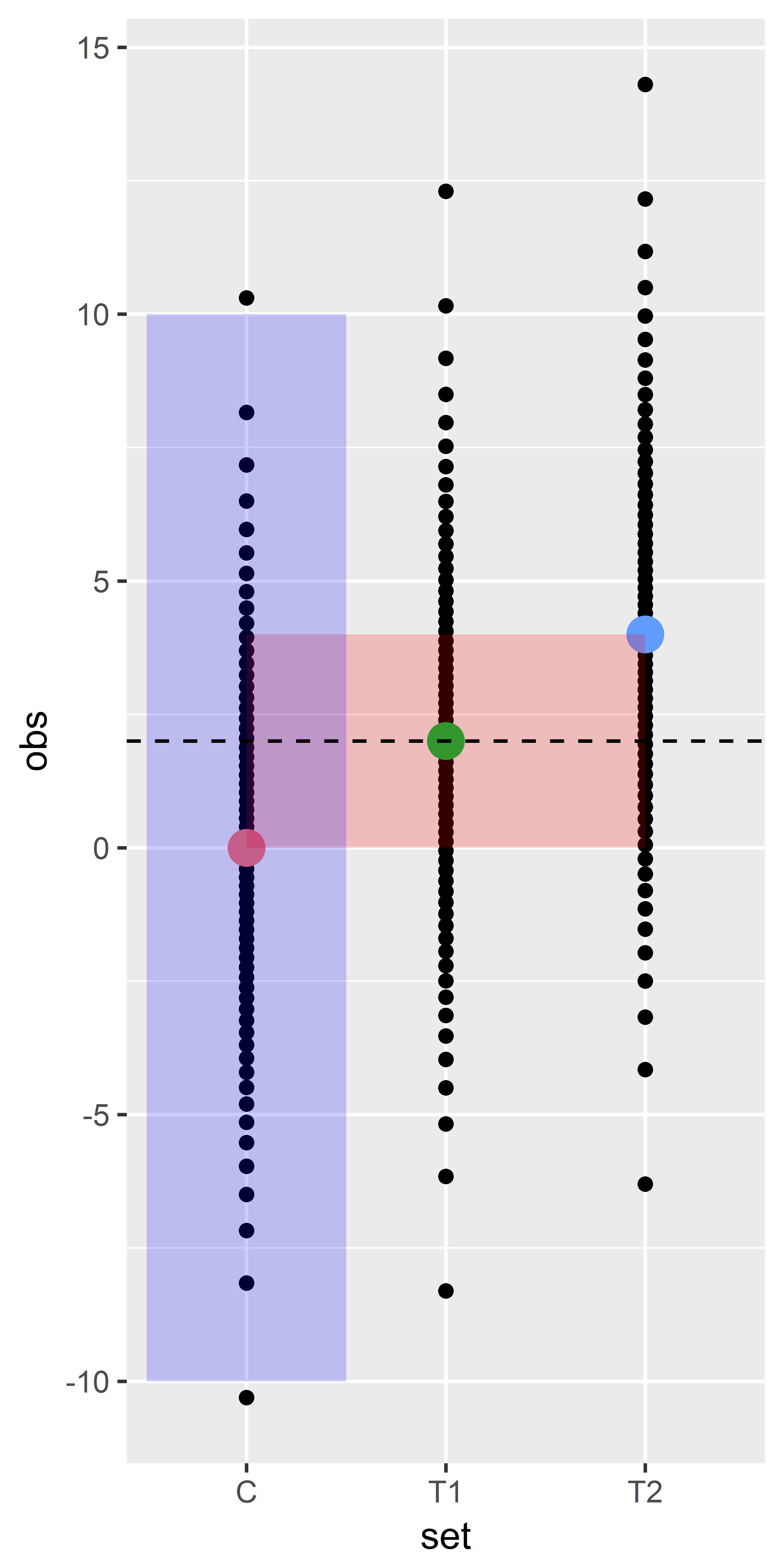
- Multiple groups &rarr; not one effect size `d`

- F-test statistic & effect size `f`, ratio of variances `$\sigma_{between}^2 / \sigma_{within}^2$`

- `$\sigma_{between}^2$` = variance between groups differences

- `$\sigma_{within}^2$` = variance within group differences

- Example: one control and two treatments 
	- `reference example` + 1 group
	- sd within each group, for all groups (C,T1,T2) = 4
	- means C=0, T1=2 and for example T2=4
]
.pull-right-30[
<img src="assets/images/anova.png" height=450></img>

]

???

---
name: omnibus

##  Multiple groups: omnibus

- Difference between some groups &rarr; at least two differ

- GPower: one-way Anova (F-test / Means, ANOVA - fixed effects, omnibus, one way)
	- effect size f, with numerator/denominator df
	- obtain sample size for `reference example`, just 2 groups C and T1 (size=64)!
	- play with sizes, how does size matter ? 
	- include third group, with mean 2, what are sample sizes (compare with 2 groups)? 
	- set third group mean to 0, how does it compare with mean 2 (think and try)? 
	- set third group mean to 4, but also vary middle group (eg., 1 or 3), does that have an effect ? 
	- change procedure: repeat for between variance 2.67 (balanced: 0, 2, 4) and within variance 16 ?

???

- GPower: one-way Anova (F-test / Means, ANOVA - fixed effects, omnibus, one way)
- Obtain sample size for `reference example`, just 2 groups C and T1 (size=64)!
	- 128, same again, despite different effect size (f) and distribution
	- size used only to include imbalance
- Include third group, with mean 2, what are sample sizes (compare with 2 groups)? 
	- effect sizes f = .236; sample size 177 (59*3), requires more observations
- Set third group mean to 0, how does it compare with mean 2 (think and try)? 
	- effect and sample size same, no difference whether big 0 group or big 2 group.
- Set third group mean to 4, but also vary middle group (eg., 1 or 3), does that have an effect ? 
	- effect sizes f = .408 (4), .425 (1/3), increase with middle group away from middle.
- Change procedure: repeat for between variance 2.67 (balanced: 0, 2, 4) and within variance 16 ? 
	- sample size 21*3=63, for f = .408 (1/7th explained = 1 between / 6 within)

---
name: omnibus_solution
exclude: false

##  Solution for multiple groups omnibus

???

---
name: multiple

##  Multiple groups: pairwise

- Assume one control, and two treatments																 
	- interested in all three pairwise comparisons &rarr; maybe Tukey
		- typically run aposteriori, after omnibus shows effect
	- use multiple t-tests with corrected `$\alpha$` for multiple testing GPower: t-tests/means difference two independent groups

- Apply Bonferroni correction for original 3 group example (0, 2, 4)
	- what samples sizes are necessary for all three pairwise tests ?
	- what if biggest difference ignored (C-T2), because know that easier to detect ? 
	- with original 64 sized groups, what is the power to detect a difference group (C-T1) (both situations above) ?

???

- GPower: t-tests/means difference two independent groups
- Apply Bonferroni correction for original 3 group example (0, 2, 4)
- What samples sizes are necessary for all three pairwise tests ?
	- 0-2 and 2-4 &rarr; d=.5, 0-4 &rarr; d=1
	- divide `$\alpha$` by 3 &rarr; .05/3=.0167
	- sample size 86 * 2 for 0-2 and 2-4, 23 * 2 for 0-4 &rarr; 86 * 3 = 258
- What if biggest difference ignored (C-T2), because know that easier to detect ? 
	- divide `$\alpha$` by 2 &rarr; .05/2=.025
	- sample size 78 * 2 for 0-2 and 2-4 &rarr; 78 * 3 = 234 (24 less)
- With original 64 sized groups, what is the power (both situations above) ? 
	- .6562 for 3 tests ( `$\alpha$` =.0167)
	- .7118 for 2 tests ( `$\alpha$` =.0250)
	- post-hoc test &rarr; power-loss (lower `$\alpha$` &rarr; higher `$\beta$`)

---
name: multiple_solution
exclude: false

##  Solution for multiple groups pairwise

???

---
name: contrasts

##  Multiple groups: contrasts

.pull-left-70[

- Contrasts are linear combinations &rarr; planned comparison
	- eg., `$1 * T1 -1 * C \neq 0$` & `$1 * T2 -1 * C \neq 0$`
	- eg., `$.5 * (1 * T1 + 1 * T2) -1 * C \neq 0$`

- Effect sizes for planned comparisons must be calculated !!
	- variance ratios (between / within)
	- standard deviation of contrasts &rarr; between variance

- Each contrast 
	- uses 1 degree of freedom
	- combines a specific number of levels

- Multiple testing correction may be appropriate 
]
.pull-right-30[

group means `$\mu_i$`  
pre-specified coefficients `$c_i$`  
sample sizes `$n_i$`  
total sample size `$N$`

`$\sigma_{contrast} = \frac{|\sum{\mu_i * c_i}|}{\sqrt{N \sum_i^k c_i^2 / n_i}}$`

]

???

---
name: contrasts_again

##  Multiple groups: contrasts (continued)

- GPower: one-way ANOVA (F-test / Means, ANOVA-fixed effects,special,main,interaction)

- Obtain effect sizes for contrasts (assume equally sized for convenience)
	- `$\sigma_{contrast}$` T1-C: `$\frac{(-1*0 + 1*2 + 0*4)}{\sqrt(2*((-1)^2+1^2+0^2))} = 1$`; `$\sigma_{error}$` = 4 &rarr; `$f$`=.25
	- `$\sigma_{contrast}$` T2-C: `$\frac{(-1*0 + 0*2 + 1*4)}{\sqrt(2*((-1)^2+0^2+1^2))} = 2$`; `$\sigma_{error}$` = 4 &rarr; `$f$`=.5
	- `$\sigma_{contrast}$` (T1+T2)/2-C: `$\frac{(-1*0 + (1/2)*2 + (1/2)*4)}{\sqrt(3*((-1)^2+(1/2)^2+(1/2)^2))} = 1.414214$`; `$\sigma_{error}$` = 4 &rarr; `$f$`=.3535

- Sample size for each contrast, each 1 df  
	- what samples sizes for either contrast 1 or contrast 2 ?
	- what samples sizes for both contrast 1 and contrast 2 combined ?
	- if taking that sample size, what will be the power for T1-T2 ?
	- what samples size for contrast 3 ?

???

- GPower: one-way ANOVA (F-test / Means, ANOVA-fixed effects,special,main,interaction)
- What samples sizes for either contrast 1 or contrast 2 ?
	- variance explained `$1^2$` or `$2^2$`
	- for T1-C `$f$` = `$\sqrt{1^2/4^2}$` = .25 = d/2 &rarr; 128 (64 C - 64 T1)
	- for T2-C `$f$` = `$\sqrt{2^2/4^2}$` = .50 = d/2 &rarr; 34 (17 C - 17 T2)
- What samples sizes for both contrast 1 and contrast 2 combined ?
	- multiple testing, consider Bonferroni correction &rarr; /2
	- for T1-C 155, for T2-C 41 &rarr; total 175 (78 C, 77 T1, 20 T2)
- If taking that sample size, what will be the power for T1-T2 ?
	- post-hoc, 77 and 20, with d=.5 and `$\alpha$` = .5 &rarr; power `$\approx$` .5
- What samples size for contrast 3 ?
	- variance contrast `$1.4142^2$`
	- 3 groups, little impact if any
	- for .5*(T1+T2) - C `$f$` = `$\sqrt{2/16}$` = .3535 &rarr; 65 (22 C, 21 T1, 22 T2)

---
name: contrasts_solution
exclude: false

##  Solution for multiple groups contrasts

???

---
name: factors

##  Multiple factors

- Multiple main effects and possibly interaction effects (eg., treatment and type)
	- main effects (average effects, additive) & interaction (factor level specific effects)
	- note: numerator degrees of freedom &rarr; main effect (nr-1), interaction (nr1-1)*(nr2-1)
	- `$\eta^2$` = `$f^2 / (1+f^2)$`, remember `$f = d/2$` for two groups
	- note: get effect sizes for two way anova: http://apps.icds.be/effectSizes/

- GPower: multiway ANOVA (F-test / Means, ANOVA-fixed effects,special,main,interaction) 
	- determine `$\eta^2$` and sample size for `reference example`, remember the between group variance ?
	- use the app: use for means only values 0 and 2, and 4 and 6 if necessary
	 for treatment use C-T1-T2, for type (second predictor) use B1-B2
		- get `$\eta^2$` for treatment effect but no type effect ? recognize `$f$` ?
		- specify such that types differ, not treatment &rarr; `$f$` and sample size ?
		- specify such that treatment effect only for one type &rarr; `$f$` and sample size ?
		- specify effect for both treatment and type, without interaction &rarr; `$f$` and sample size ?

???

- GPower: multiway ANOVA (F-test / Means, ANOVA-fixed effects,special,main,interaction)
- Determine sample size for `reference example`, remember the between group variance ?
	- between group variance 1, within 16, sample size 128 (numerator df = 2-1)
	- 2 x 2 with 0-2 &rarr; `$\eta^2$` as expected = .0588
- Get `$\eta^2$` for treatment effect but no type effect ? recognize `$f$` ?
	- 0-2-4 for both types &rarr; `$f$` = .4082 of the omnibus F-test (compare all groups)
- Specify such that types differ, not treatment &rarr; `$f$` and sample size ?
	- 0-0-0 versus 2-2-2 &rarr; `$f$` = .25 of t-test (compare two groups)
- Specify such that treatment effect only for one type &rarr; `$f$` and sample size ?
	- 0-2-4 versus 0-0-0 &rarr; `$f$` = .2041, .25 and .2041
		- detect interaction (num df = 2) = 235 total (40 per combination)
		- detect only treatment effect (num df = 2) = 235 total (79 each group, 79/2 per combination)
		- detect only type effect (num df = 1) = 128 total (64 each group, 64/3 per combination)
		- detect both both main effects = 40 each combination ~ max(79/2,64/3)
- Specify effect for both treatment and type, without interaction &rarr; `$f$` and sample size ?
	- 0-2-4 versus 2-4-6 &rarr; `$f$` = .4082, .25 and 0, sample size = 21 per combination

---
name: factors_solution
exclude: false

##  Solution for multiple factors

???

---
name: repeated

##  Repeated measures

- If repeated measures &rarr; account for correlations within

- Possible to focus on:
	- within: similar to dependent t-test for multiple measurements
	- between: group comparison, each based on multiple measurements
	- interaction: difference between changes over measurements (within)

- Correlation within unit (eg., within subject)
	- informative within unit (like paired t-test)
	- redundancy on information between units (observations less informative)

- Beware: effect size could include or exclude correlation

- GPower: repeated measures (F-test / Means, repeated measures...)
	- correlation not yet included &rarr; Options: 'as in GPower 3.0'
	- correlation already included &rarr; Options: 'as in SPSS'

???

- suggested youtube: https://www.youtube.com/watch?v=CEQUNYg80Y0

---
name: repeated_within

##  Repeated measures within

- GPower: repeated measures (F-test / Means, repeated measures within factors)

- Use effect size f = .25 (1/16 explained versus unexplained)
	- mimic dependent t-test, correlation .5 !
	- mimic independent t-test, but only use 1 group !
	- double number of groups to 2, or 4 (cor = .5), what changes ?
	- double number of measurements to 4 (cor = .5), impact ? 
	- compare impact double number of measurements for correlations .5 with .25 ?

???

- GPower: repeated measures (F-test / Means, repeated measures within factors)
- Mimic dependent t-test, correlation .5 !
	- only 1 group, 2 repeated measures, correlation .5 &rarr; 34 x 2 measurements
- Mimic independent t-test, but only use 1 group !
	- only 1 group, 2 repeated measures, correlation 0 &rarr; 65 x 2 measurements
- Double number of groups to 2, or 4 (cor = .5), what changes ?
	- number of groups not relevant for within group comparison
	- but requires estimation, changed degrees of freedom
- Double number of measurements to 4 (cor = .5), impact ? 
	- sample size reduces from 34 to 24, but 34x2=68, 24*4=96
- With 4 measurements (double) take halve the correlation (0.25), impact ? 
	- sample size 35, nearly 34
	- 2 repeated measurements with corr .5, about same sample size as 4 repeats with corr .25

---
name: repeated_within_solution
exclude: false

##  Solution for repeated measures within

???

---
name: repeated_between

##  Repeated measures between

- GPower: repeated measures (F-test / Means, repeated measures between factors)

- Use effect size f = .25 (1/16 explained versus unexplained)
	- compare 2 groups, each 2 measurements... impact on sample size when correlation 0, .25 and .5 ?
	- double number of groups to 2, or 4 (cor = .5), what changes ?
	- double number of measurements to 4 (cor = .5), impact ? 
	- compare impact number of measurements for different correlations .5 with .25 ? 
	- mimic independent t-test ?

???

- GPower: repeated measures (F-test / Means, repeated measures between factors)
- Use effect size f = .25 (1/16 explained versus unexplained)
- Compare 2 groups, each 2 measurements... impact on sample size when correlation 0, .25 and .5 ?
	- increase in correlations results in increase in sample size (redundancy)
- Double number of groups to 2, or 4 (cor = .5), what changes ?
	- increase in number of groups, small increase (estimation required) IF same effect size `$f$`
- Double number of measurements to 4 (cor = .5), impact ? 
	- increase in number of measurements, increases total number, but reduces number of units
- Compare impact number of measurements for different correlations .5 with .25 ? 
	- increase stronger if correlations stronger
- Mimic independent t-test ?
	- 128 units, if .99 correlation with fully redundant second set
	- 132 units (66*2), if 0 correlation with need to estimate four group (2x2) averages and correlation

---
name: repeated_between_solution
exclude: false

##  Solution for repeated measures between

- GPower: repeated measures (F-test / Means, repeated measures between factors)
- Use effect size f = .25 (1/16 explained versus unexplained)
- Compare 2 groups, each 2 measurements... impact on sample size when correlation 0, .25 and .5 ?
	- increase in correlations results in increase in sample size (redundancy)
- Double number of groups to 2, or 4 (cor = .5), what changes ?
	- increase in number of groups, small increase (estimation required) IF same effect size `$f$`
- Double number of measurements to 4 (cor = .5), impact ? 
	- increase in number of measurements, increases total number, but reduces number of units
- Compare impact number of measurements for different correlations .5 with .25 ? 
	- increase stronger if correlations stronger
- Mimic independent t-test ?
	- 128 units, if .99 correlation with fully redundant second set
	- 132 units (66*2), if 0 correlation with need to estimate four group (2x2) averages and correlation

???

---
name: repeated_interaction

##  Repeated measures interaction within x between

- GPower: repeated measures (F-test / Means, repeated measures within-between factors)

- Option: calculate effect sizes: http://apps.icds.be/effectSizes/
	- for sd = 4, with group with average 0-2-4, and with non-responsive (all 0): 
	- compare effect sizes for interaction with correlation .5 and 0, conclude ?
	- compare sample sizes for those 2 effect sizes with correlation .5 or 0 ?

???

- GPower: repeated measures (F-test / Means, repeated measures within-between factors)
- Option: calculate effect sizes: http://apps.icds.be/effectSizes/
- For sd = 4, with group with average 0-2-4, and with non-responsive (all 0): 
- Compare effect sizes for interaction with correlation .5 and 0, conclude ?
	- with 0 correlation &rarr; `$f$` for interaction = .25
	- with .5 correlation &rarr; `$f$` = .3536
- Compare sample sizes for those 2 effect sizes with correlation .5 or 0 ? 
	- for `$f$` = .25, sample sizes are 54x2 (cor=0) and 28x2 (cor=.5)
	- for `$f$` = .3535, sample sizes are 28x2 (cor=0) and 16x2 (cor=.5)
	- either include .5 correlation to calculate effect size OR sample size

---
name: repeated_interaction_solution
exclude: false

##  Solution for repeated measures interaction within x between

???

---
name: correlations

##  Correlations

- If comparing two independent correlations

- Use Fisher Z transformations to normalize first
	- z = .5 * log( `$\frac{1+r}{1-r}$` ) &rarr; q = z1-z2

- GPower: z-tests / correlation & regressions: 2 indep. Pearson r's 
	- with correlation coefficients .7844 and .5, what are the effect & sample sizes ? 
	- with the same difference, but stronger correlations, eg., .9844 and .7, what changes ? 
	- with the same difference, but weaker correlations, eg., .1 and .3844, what changes ?

- Note that dependent correlations are more difficult, see manual

???

- GPower: z-tests / correlation & regressions: 2 indep. Pearson r's
- With correlation coefficients .7844 and .5, what are the effect & sample sizes ? 
	- effect size q = 0.5074, sample size 64*2 = 128
	- `$.5*log((1+.7844)/(1-.7844)) - .5*log((1+.5)/(1-.5))$`
	- notice: effect size q `$\approx$` d, same sample size
- With the same difference, but stronger correlations, eg., .9844 and .7, what changes ? 
	- effect size q = 1.5556, sample size 10*2 = 20
	- same difference but bigger effect (higher correlations more easy to differentiate)
- With the same difference, but weaker correlations, eg., .1 and .3844, what changes ? 
	- effect size q = 0.3048, sample size 172*2 = 344
	- same difference, negative, and smaller effect (lower correlations more difficult to differentiate)

---
name: correlations_solution
exclude: false

##  Solution for correlations

???

---
name: proportions

##  Proportions

- If comparing two independent proportions &rarr; bounded between 0 and 1

- GPower: Fisher Exact Test (exact / proportions, difference 2 independent proportions)

- Effect sizes in odds ratio, relative risk, difference proportion
	- for odds ratio 3 and p2 = .50, what is p1 ? and for odds ratio 1/3 ?
	- what is the sample size to detect a difference for both situations ? 
	- for odds ratio 3 and p2 = .75, determine p1 and sample size, how does it compare with before ? 
	- for odds ratio 1/3 and p2 = .25, determine p1 and sample size, how does it compare with before ?
	- compare sample size for a .15 difference, at p1=.5 ?

???

- GPower: Fisher Exact Test (exact / proportions, difference 2 independent proportions)
- For odds ratio 3 and p2 = .50, what is p1 ? and for odds ratio 1/3 ?
	- odds ratio 3 &rarr; with p2 = .5 or odds_2 = 1, odds_1 = 3 thus p1 = 3/(3+1) = .75 
- What is the sample size to detect a difference for both situations ?
	- 128, same for .5 versus .25 or .75 (unlike correlation)
- For odds ratio 3 and p2 = .75, determine p1 and sample size, how does it compare with before ? 
	- p1 to .9, difference of .15, sample size increases to 220
- For odds ratio 1/3 and p2 = .25, determine p1 and sample size, how does it compare with before ?
	- p1 to .1, difference of .15, sample size increases to 220
- Compare sample size for a .15 difference, at p1=.5 ?
	- sample size even higher, to 366, increase not because smaller difference

---
name: proportions_solution
exclude: false

## Solution for proportions

- GPower: Fisher Exact Test (exact / proportions, difference 2 independent proportions)
- For odds ratio 3 and p2 = .50, what is p1 ? and for odds ratio 1/3 ?
	- odds ratio 3 &rarr; with p2 = .5 or odds_2 = 1, odds_1 = 3 thus p1 = 3/(3+1) = .75  
- What is the sample size to detect a difference for both situations ?
	- 128, same for .5 versus .25 or .75 (unlike correlation)
- For odds ratio 3 and p2 = .75, determine p1 and sample size, how does it compare with before ? 
	- p1 to .9, difference of .15, sample size increases to 220
- For odds ratio 1/3 and p2 = .25, determine p1 and sample size, how does it compare with before ?
	- p1 to .1, difference of .15, sample size increases to 220
- Compare sample size for a .15 difference, at p1=.5 ?
	- sample size even higher, to 366, increase not because smaller difference

???

---
name: proportions_exercise

##  Exercise proportions

- GPower: Fisher Exact Test (exact / proportions, difference 2 independent proportions)

.pull-left-60[

- For odds ratio = 2, with p2 reference probability .6

- Plot power over proportions .5 to 1

- Include 5 curves, sample sizes 328, 428, 528...

- With type I error .05

- Explain curve minimum, relation sample size ?

- Repeat for one-tailed, difference ?

]
.pull-right-40[

<img src="assets/images/GPowerFisher.png"></img>
]

???

- For odds ratio = 2, with p2 reference probability .6
- Plot power over proportions .5 to 1
- Include 5 curves, sample sizes 328, 428, 528...
- With type I error .05 
- Explain curve minimum, relation sample size ? 
	- power for proportion compared to reference .6
	- minimum is type I error probability
	- sample size determines impact
- Repeat for one-tailed, difference ? 
	- one-tailed, increases power (both sides !?)

---
name: proportions_exercise_solution
exclude: false

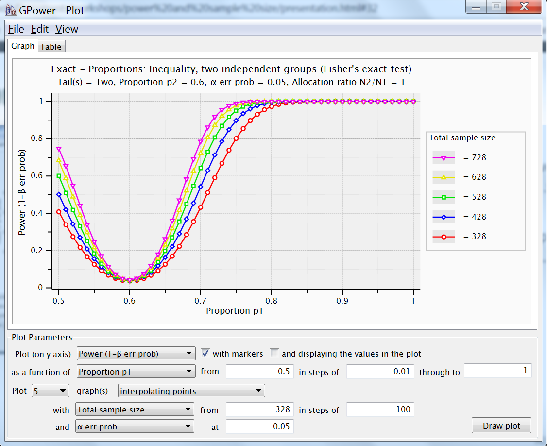
##  Solution for proportions

- GPower: Fisher Exact Test (exact / proportions, difference 2 independent proportions)

.pull-left-60[
- For odds ratio = 2, with p2 reference probability .6
- Plot power over proportions .5 to 1
- Include 5 curves, sample sizes 328, 428, 528...
- With type I error .05 
- Explain curve minimum, relation sample size ? 
	- power for proportion compared to reference .6
	- minimum is type I error probability
	- sample size determines impact
- Repeat for one-tailed, difference ? 
	- one-tailed, increases power (both sides !?)
]
.pull-right-40[
<img src="assets/images/GPowerFisher.png"></img>
]

???

---
name: proportions_dependent

##  Dependent proportions

- If comparing two dependent proportions &rarr; categorical shift
	- if only two categories, McNemar test: compare `$p_{12}$` with `$p_{21}$`
	- information from changes only &rarr; discordant pairs
	- effect size as odds ratio &rarr; ratio of discordance
	- like other exact tests, choice assignment alpha

- GPower: McNemar test (exact / proportions, difference 2 dependent proportions)
	- assume odds ratio equal to 2, equal sized, type I and II errors .05 and .2, two-way !
	- what is the sample size for .25 proportion discordant, .5, and 1  ?
	- odds ratio 1 versus .5, (prop discordant = .25), what are `$p_12$` and `$p_21$` and sample sizes ? 
	- repeat for third alpha option, and consider total sample size, what happens ?

???

- GPower: McNemar test (exact / proportions, difference 2 dependent proportions)
- Assume odds ratio equal to 2, equal sized, type I and II errors .05 and .2, two-way !
- What is the sample size for .25 proportion discordant, .5, and 1  ?
	- 288 (.25), 144 (.5), 73~144/2 (.99) &rarr; decrease in sample size with increased discordance
- Odds ratio .5 or 4, (prop discordant = .25), what are `$p_{12}$` and `$p_{21}$` and sample sizes ? 
	- same as 2 but reverse `$p_{12}$` and `$p_{21}$`, with sample size 288
	- with 4 as odds ratio, larger effect, requires smaller sample size, only 80
	- odds ratio = `$p_{12}$` / `$p_{21}$`
- Repeat for third alpha option, with odds ratio 4, what happens ? 
	- changed lower / upper critical N, lower sample size
	- BUT, is because lower power, closer to requested .8

---
name: proportions_dependent_solutions
exclude: false

##  Solution for dependent proportions

???

---
name: not_included

##  Not included

- Various statistical tests difficult to specify in GPower
	- various statistics / parametervalues that are difficult to guestimate
	- manual for more complex tests not always very elaborate

- Various statistical tests not included in GPower
	- eg., survival analysis
	- many tools online, most dedicated to a particular model

- Various statistical tests no formula to offer sample size
	- simulation may be the only tool
		- iterate many times: generate and analyze &rarr; proportion of rejections
		- generate: simulated outcome &larr; model and uncertainties
		- analyze: simulated outcome &rarr; model and parameter estimates + statistics

???

---
name: simulation

##  Simulation example t-test

```
gr <- rep(c('T','C'),64)
y <- ifelse(gr=='C',0,2)
dta <- data.frame(y=y,X=gr)
cutoff <- qt(.025,nrow(dta))
 
my_sim_function <- function(){
	dta$y <- dta$y+rnorm(length(dta$X),0,4)		# generate (with sd=4)
	res <- t.test(data=dta,y~X)					# analyze
	c(res$estimate %*% c(-1,1),res$statistic,res$p.value)
}
sims <- replicate(10000,my_sim_function())		# many iterations
dimnames(sims)[[1]] <- c('diff','t.stat','p.val')

mean(sims['p.val',] < .05)	# p-values	0.8029
mean(sims['t.stat',] < cutoff)	# t-statistics 0.8029
mean(sims['diff',] > sd(sims['diff',])*cutoff*(-1))	# differences 0.8024
```

???

---
name: focus

##  Focus / simplify

- Complex statistical models
	- simulate BUT it requires programming and a thorough understanding of the model
	- alternative: focus on essential elements &rarr; simplify the aim

- Sample size calculations (design) for simpler research aim
	- not necessarily equivalent to final statistical testing / estimation
	- requires justification to convince yourself and/or reviewers
		- successful already if simple aim is satisfied
		- ignored part is not too costly

- Example: 
	- statistics: group difference evolution 4 repeated measurements &rarr; mixed model
	- focus: difference treatment and control last time point is essential &rarr; t-test
	- argument: first 3 measurements low cost, interesting to see change

???

---
name: conclusion

##  Conclusion

- Sample size calculation is a design issue, not a statistical one

- Building blocks: sample & effect sizes, type I & II errors
	- establish any of these building blocks, conditional on the rest

- Effect sizes express the amount of signal compared to the background noise

- GPower deals with not too complex models
	- more complex complex models imply more complex specification
	- simplify using a focus, if justifiable &rarr; then GPower can get you a long way

---

Methodological and statistical support to help make a difference

- SQUARE provides complementary support in methodology and statistics to our research community, for both individual researchers and research groups, in order to get the best out of them

- SQUARE aims to address all questions related to quantitative research, and to further enhance the quality of both the research and how it is communicated

website: https://square.research.vub.be/ includes information on who we serve, and how

booking: https://square.research.vub.be/bookings for individual consultations